<?xml version="1.0" encoding="utf-8"?><feed xmlns="http://www.w3.org/2005/Atom" ><generator uri="https://jekyllrb.com/" version="3.10.0">Jekyll</generator><link href="https://hellojais.github.io/feed.xml" rel="self" type="application/atom+xml" /><link href="https://hellojais.github.io/" rel="alternate" type="text/html" /><updated>2026-07-10T02:31:43+00:00</updated><id>https://hellojais.github.io/feed.xml</id><title type="html">Santosh Jaiswal</title><subtitle>Research blog on machine learning and world models</subtitle><author><name>Santosh Jaiswal</name></author><entry><title type="html">From Laptop to Blackwell: Scaling an AV World Model with Omnissa Horizon VDI</title><link href="https://hellojais.github.io/2026/07/09/scaling-av-world-model-blackwell-vdi.html" rel="alternate" type="text/html" title="From Laptop to Blackwell: Scaling an AV World Model with Omnissa Horizon VDI" /><published>2026-07-09T00:00:00+00:00</published><updated>2026-07-09T00:00:00+00:00</updated><id>https://hellojais.github.io/2026/07/09/scaling-av-world-model-blackwell-vdi</id><content type="html" xml:base="https://hellojais.github.io/2026/07/09/scaling-av-world-model-blackwell-vdi.html"><![CDATA[<p><em>This post is Part 2 of a series. Part 1 covers the minDrive-JEPA paper, a
transformer-based latent world model for autonomous vehicles that I trained on a
MacBook and published on arXiv. If you haven’t read it, the short version: instead
of predicting raw pixels or coordinates, the model learns to predict in <strong>latent
space</strong> using a JEPA objective. The result is a “surprise score”, a real-valued
signal per scenario that tells you how unexpected a driving situation was. Part 1
is at <a href="https://arxiv.org/abs/2606.28383">arXiv:2606.28383</a>. This post is about what
happened when I tried to scale it.</em></p>

<hr />

<h2 id="the-wall">The Wall</h2>

<p>The paper model was trained on nuPlan mini, roughly 1,000 driving scenarios. That
was enough to validate the idea. But autonomous vehicle systems need to handle the
full distribution of real-world driving: dense urban intersections, highway merges,
pedestrian crossings across cities on two continents. The full nuPlan dataset
is 63,000 scenarios. Add Argoverse 2 and you’re at <strong>263,000</strong>.</p>

<p>My MacBook M5 Max is a genuinely powerful machine. But it has hard limits for this
kind of work:</p>

<ul>
  <li><strong>No FP8 tensor cores.</strong> Apple Silicon uses MPS, not CUDA. FP8, the precision
that gives Blackwell GPUs 2× the throughput of BF16, doesn’t exist on it.
Training at FP32 on MPS for 200 epochs over 263K scenarios would have taken days,
not hours. And FP8 isn’t just a software flag. It’s a capability that lives in
the silicon. You can’t emulate it on a laptop.</li>
  <li><strong>No FlashAttention.</strong> The memory-efficient attention kernel that makes large
transformer batches tractable is CUDA-only.</li>
  <li><strong>Storage.</strong> The raw datasets are hundreds of gigabytes. That’s NFS territory,
not a local SSD.</li>
  <li><strong>Batch size.</strong> Chinchilla scaling tells you that a 38.7M parameter model needs
roughly 263K training samples to avoid overfitting. Getting there requires a batch
size of 512 and 48GB of GPU memory, a configuration that doesn’t fit on any
laptop.</li>
</ul>

<p>The model I wanted to train was physically impossible on the hardware I had.</p>

<hr />

<h2 id="why-horizon-vdi-was-the-right-answer">Why Horizon VDI Was the Right Answer</h2>

<p>I’ve been engineering Omnissa Horizon VDI deployments for several years. When I hit
this wall, the solution was already in front of me.</p>

<p>Horizon VDI with <strong>NVIDIA AI-Ready vWorkstation (vWS)</strong> lets you provision a
GPU-backed virtual machine on demand, connected to shared NFS storage, running a
full CUDA stack, accessible from any endpoint. Critically, when the job is done you
<strong>release the GPU back to the shared pool</strong>. You don’t own dedicated hardware. You
borrow exactly what you need, for exactly as long as you need it.</p>

<p>For this project, that meant:</p>

<table>
  <thead>
    <tr>
      <th>Component</th>
      <th>Spec</th>
    </tr>
  </thead>
  <tbody>
    <tr>
      <td>GPU</td>
      <td>RTX Pro 6000 Blackwell, MIG 2g.48gb slice, 51.2GB vRAM</td>
    </tr>
    <tr>
      <td>Architecture</td>
      <td>SM 12.0 (Blackwell)</td>
    </tr>
    <tr>
      <td>Driver</td>
      <td>580.126.09</td>
    </tr>
    <tr>
      <td>CUDA</td>
      <td>12.8</td>
    </tr>
    <tr>
      <td>cuDNN</td>
      <td>9.19.0</td>
    </tr>
    <tr>
      <td>PyTorch</td>
      <td>2.11.0+cu128</td>
    </tr>
    <tr>
      <td>Storage</td>
      <td>2TB NFS volume (datasets + checkpoints)</td>
    </tr>
  </tbody>
</table>

<p>The NVIDIA AI vWS SDK unlocked the full Blackwell stack out of the box: CUTLASS BF16
kernels, FlashAttention, and FP8 tensor cores. These are capabilities tied to SM 12.0
silicon and would require significant infrastructure investment to replicate any other
way.</p>

<p>One important point on hypervisor flexibility: <strong>Horizon is hypervisor-agnostic</strong>.
This deployment ran on vSphere, but the same setup can work identically on Nutanix,
OpenStack, and OpenShift. The developer experience is the same regardless of what
infrastructure is underneath.</p>

<p>For enterprise customers thinking about AI developer productivity: this is exactly the
model. Data scientists and ML engineers get Blackwell-class compute on demand through
their standard VDI solution. IT provisions it, monitors it, and reclaims it. No one
buys a $10,000 workstation that sits idle between experiments.</p>

<hr />

<h2 id="what-the-project-did">What the Project Did</h2>

<h3 id="data-pipeline">Data Pipeline</h3>

<p>The first task was converting raw data into a format the model could consume. nuPlan
stores scenarios as SQLite <code class="language-plaintext highlighter-rouge">.db</code> files across four cities (Boston, Pittsburgh,
Singapore, mini split). Argoverse 2 uses Parquet. A parallel preprocessing pipeline
converted both formats into normalized tensors of shape <code class="language-plaintext highlighter-rouge">[50, 21, 6]</code>:</p>

<ul>
  <li><strong>50</strong> timesteps (subsampled from raw data)</li>
  <li><strong>21</strong> agents (ego vehicle + 20 nearest agents)</li>
  <li><strong>6</strong> features per agent: position (x, y), velocity (vx, vy), heading, agent type</li>
</ul>

<p>The pipeline ran at <strong>2,238 scenarios per second</strong> on the Blackwell VM, processing
all 263,000 scenarios in under two minutes.</p>

<h3 id="model-architecture">Model Architecture</h3>

<p>The model is a scaled-up version of the minDrive-JEPA paper architecture:</p>

<table>
  <thead>
    <tr>
      <th>Parameter</th>
      <th>Paper (minDrive-JEPA)</th>
      <th>This project</th>
    </tr>
  </thead>
  <tbody>
    <tr>
      <td>d_model</td>
      <td>128</td>
      <td>512</td>
    </tr>
    <tr>
      <td>Attention heads</td>
      <td>4</td>
      <td>8</td>
    </tr>
    <tr>
      <td>Encoder layers</td>
      <td>4</td>
      <td>8</td>
    </tr>
    <tr>
      <td>Predictor layers</td>
      <td>2</td>
      <td>4</td>
    </tr>
    <tr>
      <td>Total parameters</td>
      <td>~1.3M</td>
      <td><strong>38.7M</strong></td>
    </tr>
    <tr>
      <td>Training data</td>
      <td>~1K scenarios</td>
      <td><strong>263K scenarios</strong></td>
    </tr>
    <tr>
      <td>Training precision</td>
      <td>FP32 (MPS)</td>
      <td><strong>FP8/BF16 (Blackwell)</strong></td>
    </tr>
  </tbody>
</table>

<p>The model size was chosen using Chinchilla scaling: 38.7M parameters requires roughly
263K training samples to converge without overfitting.</p>

<h3 id="training-and-fp8">Training and FP8</h3>

<p>Training ran for 200 epochs at batch size 512.</p>

<p>Here is where FP8 matters in practice:</p>

<blockquote>
  <p><em>FP8 tensor cores on Blackwell perform roughly 2× more floating-point operations
per second than BF16, and use half the memory per weight. That’s not a software
optimization. It’s physics.</em></p>
</blockquote>

<p>This is why the model trained in <strong>5 hours and 42 minutes</strong> at <strong>11.5 TFLOPS</strong>
sustained throughput, using CUTLASS BF16 kernels and FlashAttention. The equivalent
FP32 run on the same hardware would have taken over a day. On an M5 Max it wouldn’t
have been feasible at all.</p>

<p>The end-user implication: FP8 let us train a model that would have taken 2 days on
FP32 in under 6 hours, not by changing the algorithm, just by using the right
hardware precision.</p>

<h3 id="cross-dataset-transfer-study">Cross-Dataset Transfer Study</h3>

<p>Once training was done, I ran a controlled experiment: train on nuPlan only (63K
scenarios, one geography), then evaluate on held-out Argoverse 2 validation scenarios
(cities the model had never seen). Then repeat with a combined nuPlan + AV2 model
trained on the same 63K scenario budget, so the only variable that changes is
geographic diversity, not data volume.</p>

<table>
  <thead>
    <tr>
      <th>Model</th>
      <th>Training data</th>
      <th>Mean surprise (AV2 val)</th>
    </tr>
  </thead>
  <tbody>
    <tr>
      <td>nuPlan-only</td>
      <td>63K, one geography</td>
      <td>0.273</td>
    </tr>
    <tr>
      <td>Combined (nuPlan + AV2)</td>
      <td>63K, two geographies</td>
      <td><strong>0.228</strong></td>
    </tr>
  </tbody>
</table>

<p>At identical data scale, combined training reduced mean surprise by <strong>16.5%</strong> (mean of
three seeds). Training on geographic diversity makes the model a better predictor of
driving behaviour it hasn’t seen before.</p>

<h3 id="demo">Demo</h3>

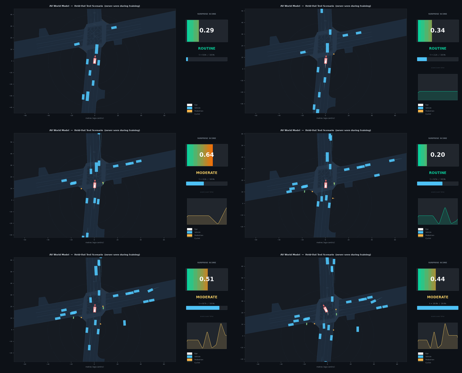
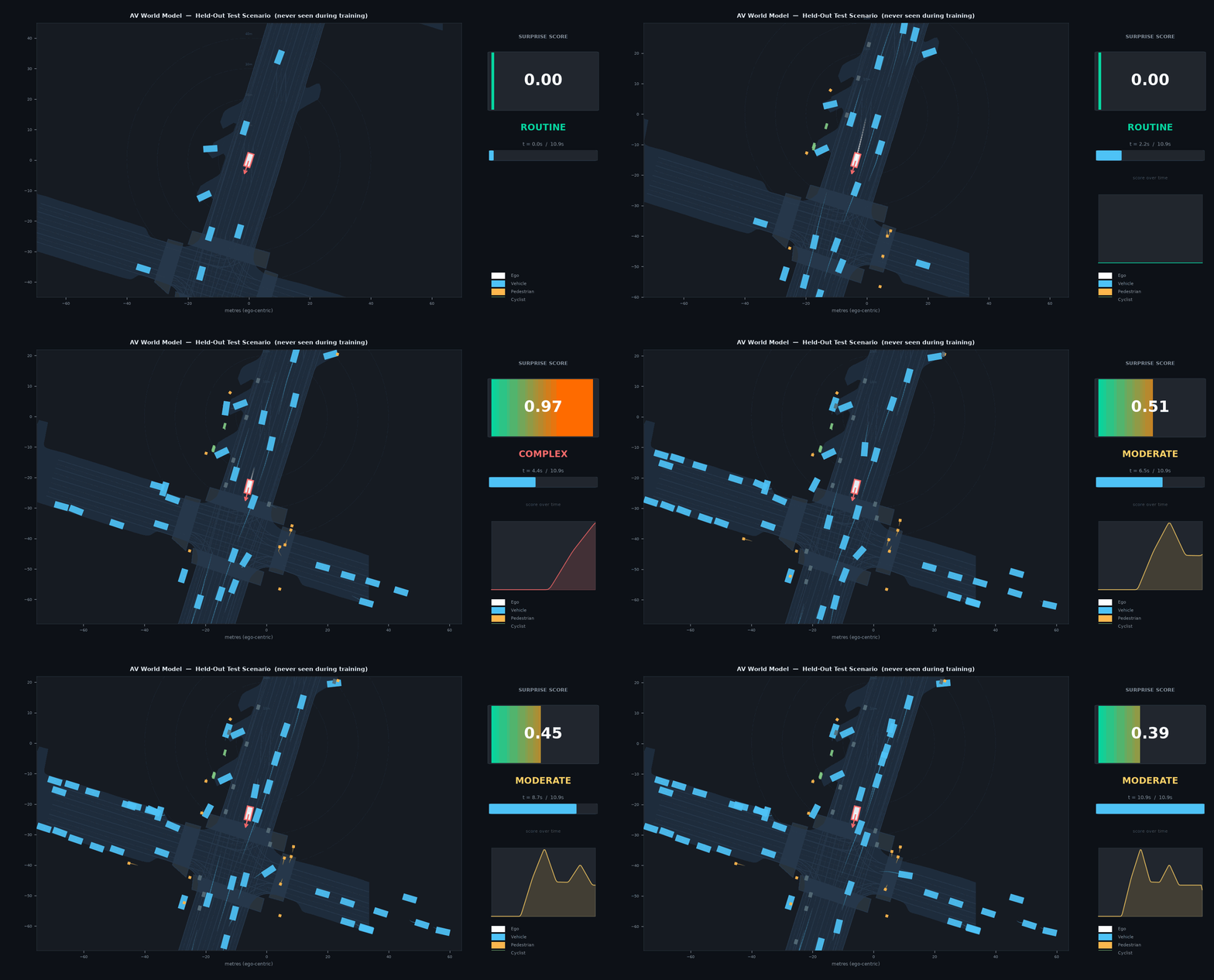
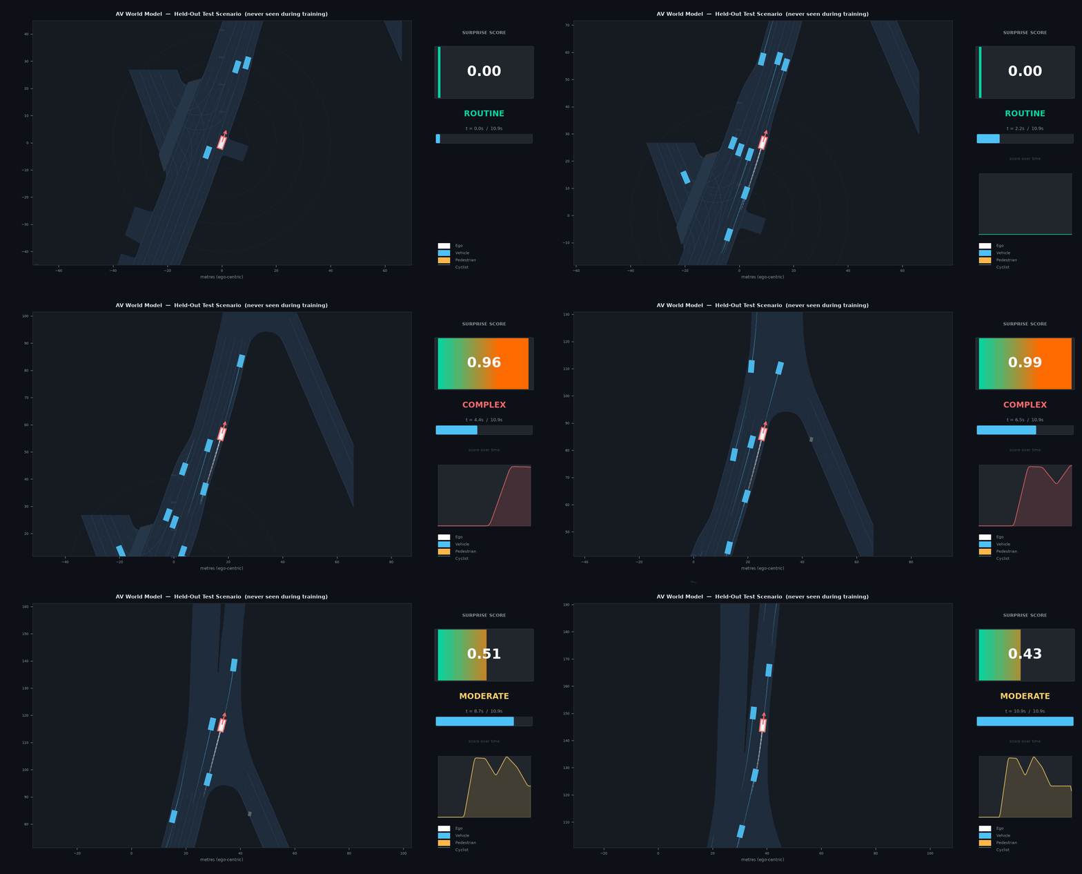
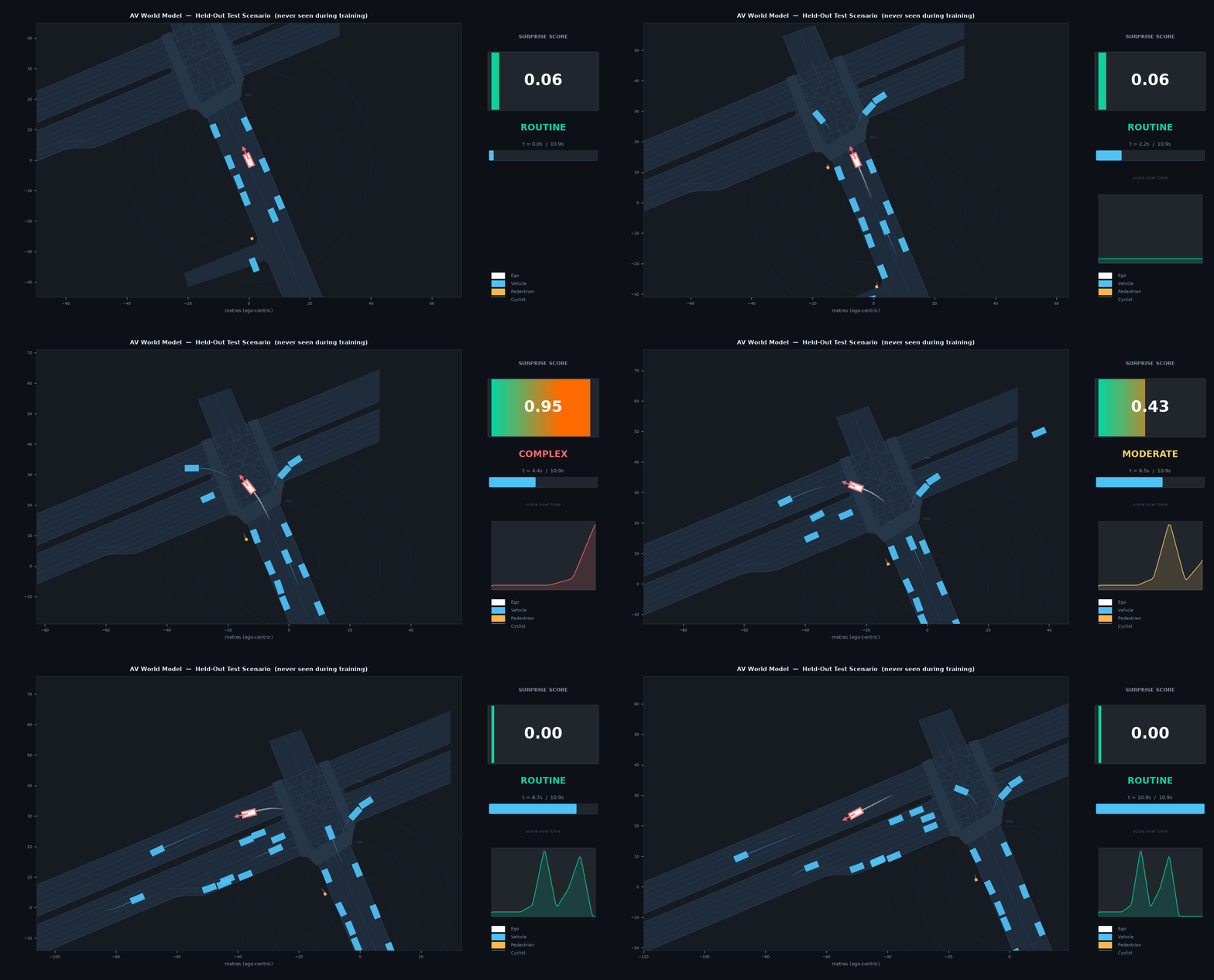
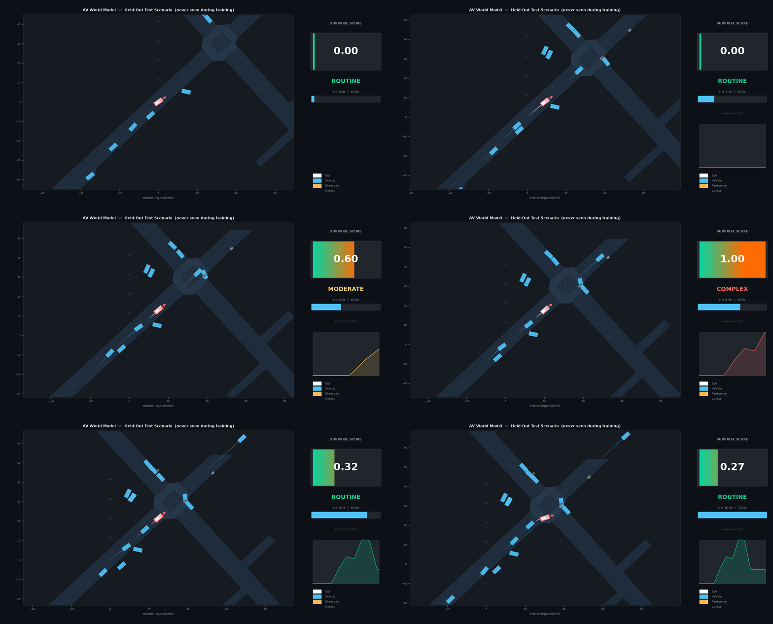
<p>The surprise score is interpretable; it’s not just a training metric. The animations
below show the model running on real held-out AV2 scenarios. The score bar turns red
when the model is surprised. It spikes at complex intersections and unexpected agent
behaviour, and stays low on routine highway driving.</p>

<p><img src="/assets/images/demo_final_172538.gif" alt="Surprise score on a held-out AV2 scenario" /></p>

<p><img src="/assets/images/demo_final_57378.gif" alt="Surprise score on a held-out AV2 scenario" /></p>

<p><img src="/assets/images/demo_final_187081.gif" alt="Surprise score on a held-out AV2 scenario" /></p>

<p><img src="/assets/images/demo_final_139387.gif" alt="Surprise score on a held-out AV2 scenario" /></p>

<p><img src="/assets/images/demo_final_57843.gif" alt="Surprise score on a held-out AV2 scenario" /></p>

<hr />

<h2 id="who-this-is-for">Who This Is For</h2>

<p>This project sits at the intersection of three audiences:</p>

<p><strong>AV researchers</strong> who want to study scene complexity and model generalization across
datasets. The surprise score gives you a cheap, differentiable proxy for “how hard
is this scenario.”</p>

<p><strong>ML platform engineers</strong> who need a concrete, reproducible example of what enterprise
GPU-on-demand looks like end-to-end: data on NFS, model in PyTorch, training on a
vWS-provisioned Blackwell VM, results reproduced by anyone with:</p>
<div class="language-bash highlighter-rouge"><div class="highlight"><pre class="highlight"><code><span class="nb">source </span>local.env
python scripts/train.py <span class="nt">--config</span> configs/combined.yaml
</code></pre></div></div>

<p><strong>Enterprise IT and VDI architects</strong> evaluating whether Horizon + NVIDIA AI vWS can
support serious AI workloads for internal developer teams. This project is evidence
that it can. Not a proof-of-concept toy, but a published research result with
263K training samples and a 38.7M parameter model trained to convergence.</p>

<p>The code is open-source at <a href="https://github.com/hellojais/av-worldmodel">github.com/hellojais/av-worldmodel</a>.<br />
The paper is at <a href="https://arxiv.org/abs/2606.28383">arXiv:2606.28383</a>.</p>]]></content><author><name>Santosh Jaiswal</name></author><category term="machine-learning" /><category term="autonomous-vehicles" /><category term="jepa" /><category term="gpu" /><category term="vdi" /><category term="horizon" /><summary type="html"><![CDATA[This post is Part 2 of a series. Part 1 covers the minDrive-JEPA paper, a transformer-based latent world model for autonomous vehicles that I trained on a MacBook and published on arXiv. If you haven’t read it, the short version: instead of predicting raw pixels or coordinates, the model learns to predict in latent space using a JEPA objective. The result is a “surprise score”, a real-valued signal per scenario that tells you how unexpected a driving situation was. Part 1 is at arXiv:2606.28383. This post is about what happened when I tried to scale it.]]></summary></entry><entry><title type="html">V-JEPA 2 on UCF-101: Backbone Generalizes, SSv2 Head Is the Bottleneck</title><link href="https://hellojais.github.io/machine-learning/world-models/representation-learning/2026/05/31/vjepa2-live-probing-representations.html" rel="alternate" type="text/html" title="V-JEPA 2 on UCF-101: Backbone Generalizes, SSv2 Head Is the Bottleneck" /><published>2026-05-31T00:00:00+00:00</published><updated>2026-05-31T00:00:00+00:00</updated><id>https://hellojais.github.io/machine-learning/world-models/representation-learning/2026/05/31/vjepa2-live-probing-representations</id><content type="html" xml:base="https://hellojais.github.io/machine-learning/world-models/representation-learning/2026/05/31/vjepa2-live-probing-representations.html"><![CDATA[<blockquote>
  <p><strong>Author:</strong> Santosh Jaiswal (<a href="https://github.com/hellojais">@hellojais</a>)<br />
<strong>Code:</strong> <a href="https://github.com/hellojais/vjepa2-live">hellojais/vjepa2-live</a><br />
<strong>Model:</strong> <a href="https://huggingface.co/qubvel-hf/vjepa2-vitl-fpc16-256-ssv2">qubvel-hf/vjepa2-vitl-fpc16-256-ssv2</a><br />
<strong>Dataset:</strong> UCF-101 (1,059 clips, 101 action classes)<br />
<strong>Hardware:</strong> MacBook Pro M5 Max, MPS backend, no CUDA</p>
</blockquote>

<hr />

<h2 id="tldr">TL;DR</h2>

<p>V-JEPA 2’s frozen backbone achieves 98.2% ± 1.0% linear probe accuracy
on UCF-101, a dataset it was never trained on. The SSv2 classification
head, by contrast, produces low-confidence or semantically mismatched
predictions for 42% of UCF-101 classes. All four “blind spot” classes
that the SSv2 head fails on completely (PoleVault, SalsaSpin,
WritingOnBoard, Surfing) achieve 100% linear probe accuracy on the same
frozen embeddings. The backbone is not the bottleneck. The classification
head’s fixed 174-word SSv2 vocabulary is.</p>

<hr />

<h2 id="motivation">Motivation</h2>

<p>V-JEPA 2 is pre-trained self-supervised: it learns by predicting
missing spatio-temporal patches in embedding space, with no labels.
A classification head is then fine-tuned on Something-Something v2
(SSv2), a dataset of 174 hand-object interaction categories.</p>

<p>The pre-training and the fine-tuning are separate stages with
separate objectives. This raises a practical question for anyone
considering adapting V-JEPA 2 to a new domain: when the model
underperforms on out-of-distribution video, is the problem in the
backbone representations or in the classification head’s limited
vocabulary? The answer determines whether you need to fine-tune the
backbone (expensive, requires data) or simply replace the head
(cheap, requires very little data).</p>

<p>This study answers that question systematically on UCF-101.</p>

<hr />

<h2 id="setup">Setup</h2>

<p><strong>Model:</strong> qubvel-hf/vjepa2-vitl-fpc16-256-ssv2, ViT-L backbone,
325M parameters, SSv2 classification head (174 classes). Used frozen
throughout. No fine-tuning at any stage.</p>

<p><strong>Dataset:</strong> UCF-101, 101 action categories, ~10 videos per class,
1,059 clips total. UCF-101 has no overlap with SSv2’s label space.</p>

<p><strong>Hardware:</strong> MacBook Pro M5 Max, 68GB unified memory, PyTorch 2.12
MPS backend. All phases run locally, no cloud, no CUDA.</p>

<p><strong>Pipeline:</strong> Four phases, each building on the previous:</p>

<table>
  <thead>
    <tr>
      <th>Phase</th>
      <th>What it does</th>
      <th>Output</th>
    </tr>
  </thead>
  <tbody>
    <tr>
      <td>1</td>
      <td>Live webcam inference, MPS validation</td>
      <td>~10fps end-to-end</td>
    </tr>
    <tr>
      <td>2</td>
      <td>Zero-shot inference on 1,059 UCF-101 videos</td>
      <td>Per-class behavior classification</td>
    </tr>
    <tr>
      <td>3</td>
      <td>Backbone embedding extraction + 4 hypothesis tests</td>
      <td>(1059, 1024) float32 embeddings</td>
    </tr>
    <tr>
      <td>4</td>
      <td>Linear probe on frozen embeddings</td>
      <td>Per-class accuracy across 101 classes</td>
    </tr>
  </tbody>
</table>

<hr />

<h2 id="phase-2-zero-shot-behavior-on-ucf-101">Phase 2: Zero-Shot Behavior on UCF-101</h2>

<p>Running the frozen model on all 1,059 UCF-101 videos and classifying
each UCF class by its prediction pattern produced three behavior
categories:</p>

<table>
  <thead>
    <tr>
      <th>Behavior</th>
      <th>Classes</th>
      <th>Description</th>
    </tr>
  </thead>
  <tbody>
    <tr>
      <td>HIGH_CONF_CONSISTENT</td>
      <td>34</td>
      <td>Confidently maps to one SSv2 concept</td>
    </tr>
    <tr>
      <td>HIGH_CONF_INCONSISTENT</td>
      <td>25</td>
      <td>High confidence, inconsistent SSv2 labels</td>
    </tr>
    <tr>
      <td>LOW_CONF_SCATTERED</td>
      <td>42</td>
      <td>Low confidence, no dominant SSv2 label</td>
    </tr>
  </tbody>
</table>

<p>Three SSv2 physics primitives dominated predictions across all 101
classes: “Hitting” (154 videos), “Throwing” (133), “Spinning” (98).
The SSv2 head’s response to out-of-distribution video collapses
to a small set of motion archetypes.</p>

<p>The HIGH_CONF_CONSISTENT mappings are the most informative. The
model is confident and consistent, but the SSv2 labels it assigns
reveal what it actually encoded:</p>

<table>
  <thead>
    <tr>
      <th>UCF Class</th>
      <th>SSv2 Prediction</th>
      <th>Confidence</th>
    </tr>
  </thead>
  <tbody>
    <tr>
      <td>PlayingDhol</td>
      <td>“Hitting [something] with [something]”</td>
      <td>0.834</td>
    </tr>
    <tr>
      <td>HulaHoop</td>
      <td>“Spinning [something] so it continues spinning”</td>
      <td>0.808</td>
    </tr>
    <tr>
      <td>WalkingWithDog</td>
      <td>“Moving away from [something] with your camera”</td>
      <td>0.718</td>
    </tr>
    <tr>
      <td>CuttingInKitchen</td>
      <td>“Spreading [something] onto [something]”</td>
      <td>0.695</td>
    </tr>
    <tr>
      <td>CleanAndJerk</td>
      <td>“Lifting [something] up completely”</td>
      <td>0.616</td>
    </tr>
  </tbody>
</table>

<p>WalkingWithDog → “Moving away from something with your camera” is
a clean example of JEPA encoding working as intended. The model
has no concept of “dog” as a subject. It encodes the camera-relative
motion pattern (scene receding as you walk forward) and maps it
to the nearest SSv2 spatial-motion concept. Object identity is absent.
Relational motion is present.</p>

<p>The four worst-performing classes share a structural property: they
all involve whole-body or tool-mediated motion with no clear
hand-object interaction. SSv2 is entirely tabletop hand-object
interactions. These classes fall outside its learned physics
vocabulary entirely.</p>

<hr />

<h2 id="phase-3-embedding-analysis">Phase 3: Embedding Analysis</h2>

<h3 id="baseline-same-class-vs-different-class-similarity">Baseline: Same-Class vs Different-Class Similarity</h3>

<p>Extracting the frozen ViT-L backbone embeddings (before the
classification head) for all 1,059 videos gives a (1059, 1024)
float32 array. The first diagnostic:</p>

<table>
  <thead>
    <tr>
      <th>Similarity type</th>
      <th>Cosine similarity</th>
    </tr>
  </thead>
  <tbody>
    <tr>
      <td>Same UCF class</td>
      <td>0.93</td>
    </tr>
    <tr>
      <td>Different UCF class</td>
      <td>0.59</td>
    </tr>
  </tbody>
</table>

<p>A 0.34 gap on action classes the backbone was never trained to
distinguish. The backbone is organizing UCF-101 videos by action
category without any UCF supervision signal.</p>

<h3 id="embedding-space-structure">Embedding Space Structure</h3>

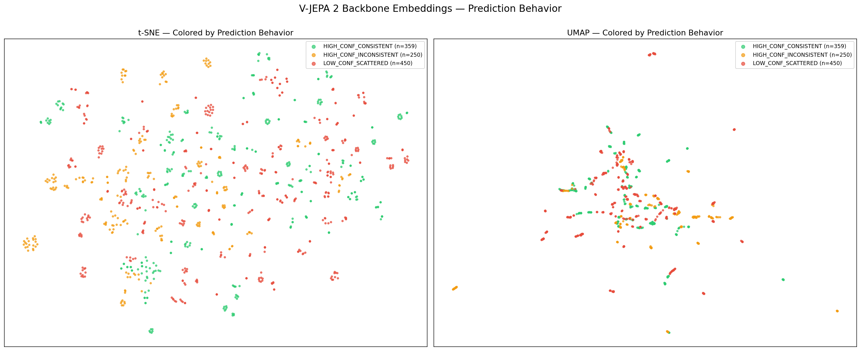
<p>t-SNE and UMAP on the 1024-dim embeddings show behavior categories
occupying distinct regions of embedding space. 94 unique SSv2 labels
were predicted across 101 UCF classes, confirming the backbone
separates most UCF classes into distinct embedding regions.</p>

<p><img src="/assets/images/vjepa2_behavior_clusters.png" alt="Behavior clusters in embedding space" />
<em>t-SNE and UMAP colored by behavior category. GREEN = HIGH_CONF_CONSISTENT, YELLOW = HIGH_CONF_INCONSISTENT, RED = LOW_CONF_SCATTERED. The three categories occupy partially separable regions, consistent with the 0.93 same-class cosine similarity baseline.</em></p>

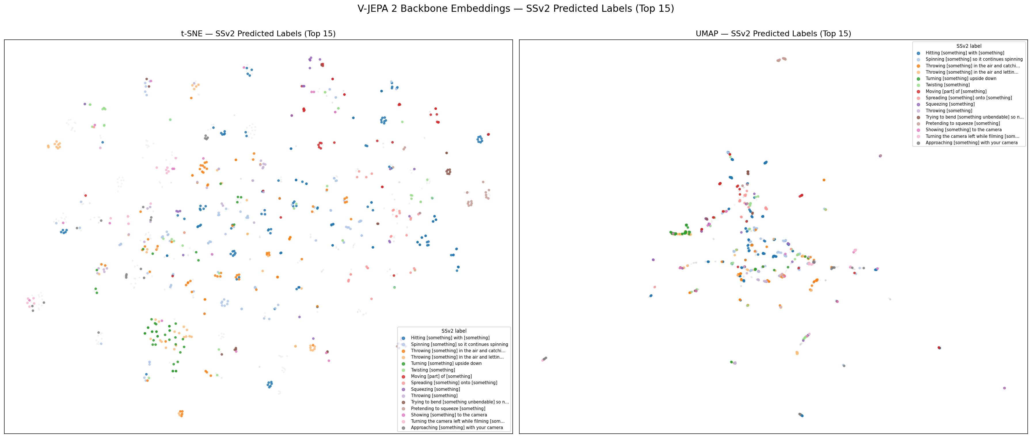
<p>The SSv2 label regions plot shows which physics primitives dominate
which areas of embedding space:</p>

<p><img src="/assets/images/vjepa2_ssv2_label_regions.png" alt="SSv2 label regions" />
<em>Top 15 SSv2 predicted labels overlaid on UMAP. “Hitting”, “Throwing”, and “Spinning” dominate large contiguous regions. Gray points are classes predicted as less frequent SSv2 labels.</em></p>

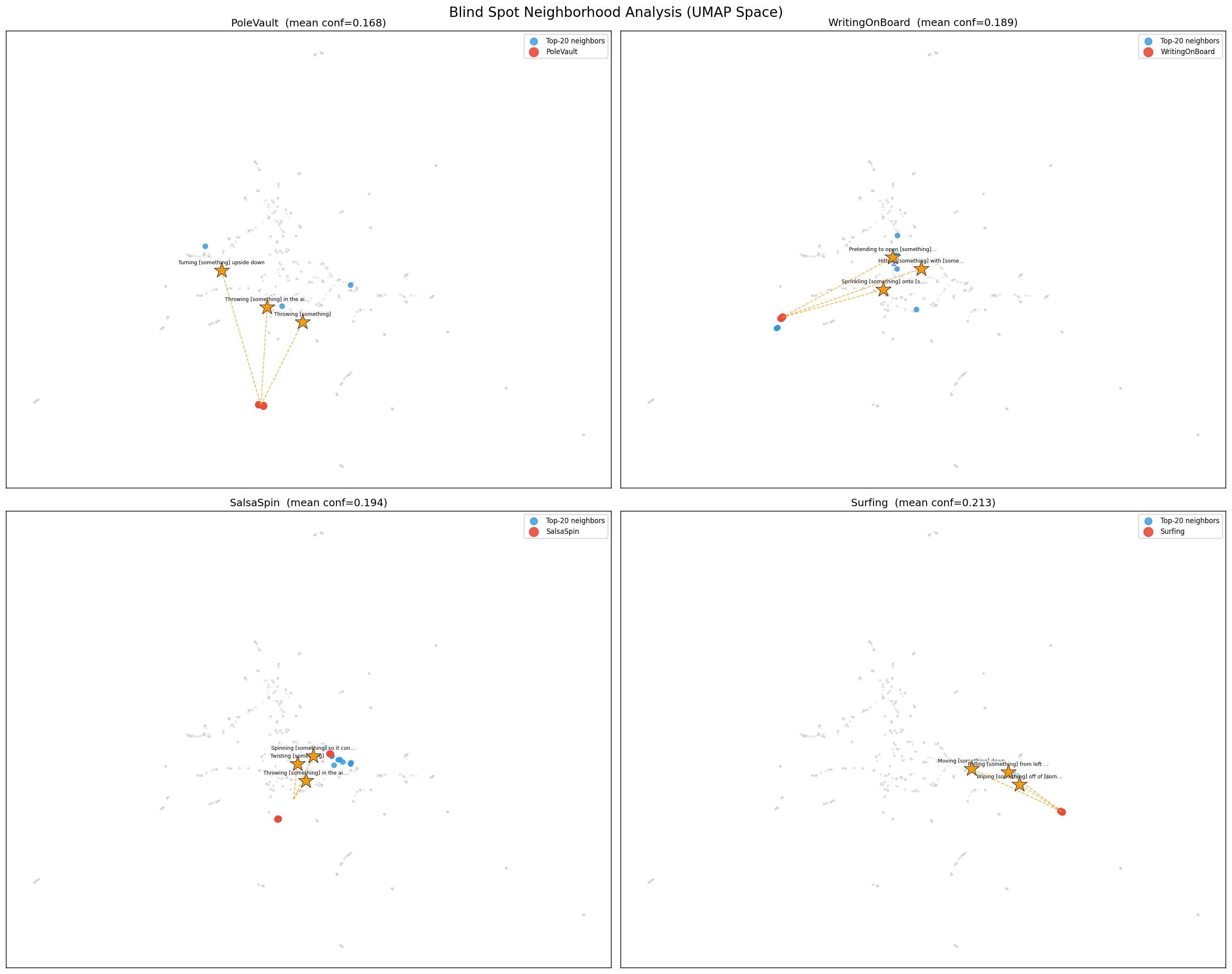
<h3 id="the-blind-spot-cluster">The Blind Spot Cluster</h3>

<p>The four lowest-confidence UCF classes cluster together in embedding
space rather than scattering randomly. They form a coherent region
with no close SSv2 centroid neighbors, a structurally isolated
“whole-body motion without hand-object interaction” region:</p>

<table>
  <thead>
    <tr>
      <th>Class</th>
      <th>SSv2 Mapping</th>
      <th>Structural reason</th>
    </tr>
  </thead>
  <tbody>
    <tr>
      <td>PoleVault</td>
      <td>“Turning upside down”</td>
      <td>Body inversion misread as object inversion</td>
    </tr>
    <tr>
      <td>SalsaSpin</td>
      <td>“Spinning something”</td>
      <td>Rotation with no hand-object contact</td>
    </tr>
    <tr>
      <td>Surfing</td>
      <td>“Wiping something off”</td>
      <td>Lateral body sweep misread as wiping</td>
    </tr>
    <tr>
      <td>WritingOnBoard</td>
      <td>“Sprinkling something”</td>
      <td>Arm arc misread as dispersal</td>
    </tr>
  </tbody>
</table>

<p><img src="/assets/images/vjepa2_blind_spot_analysis.png" alt="Blind spot neighborhood analysis" />
<em>Each blind-spot class shown in red with its 20 nearest embedding neighbors in blue. Lines connect each class centroid to its nearest SSv2 concept centroids (stars). All four blind-spot classes cluster together and share nearest neighbors; they form a coherent isolated region, not random noise.</em></p>

<p>The model has no “unknown” output. It forces every input onto the
nearest SSv2 physics primitive regardless of fit quality.</p>

<h3 id="hitting-is-a-spurious-catch-all">“Hitting” Is a Spurious Catch-All</h3>

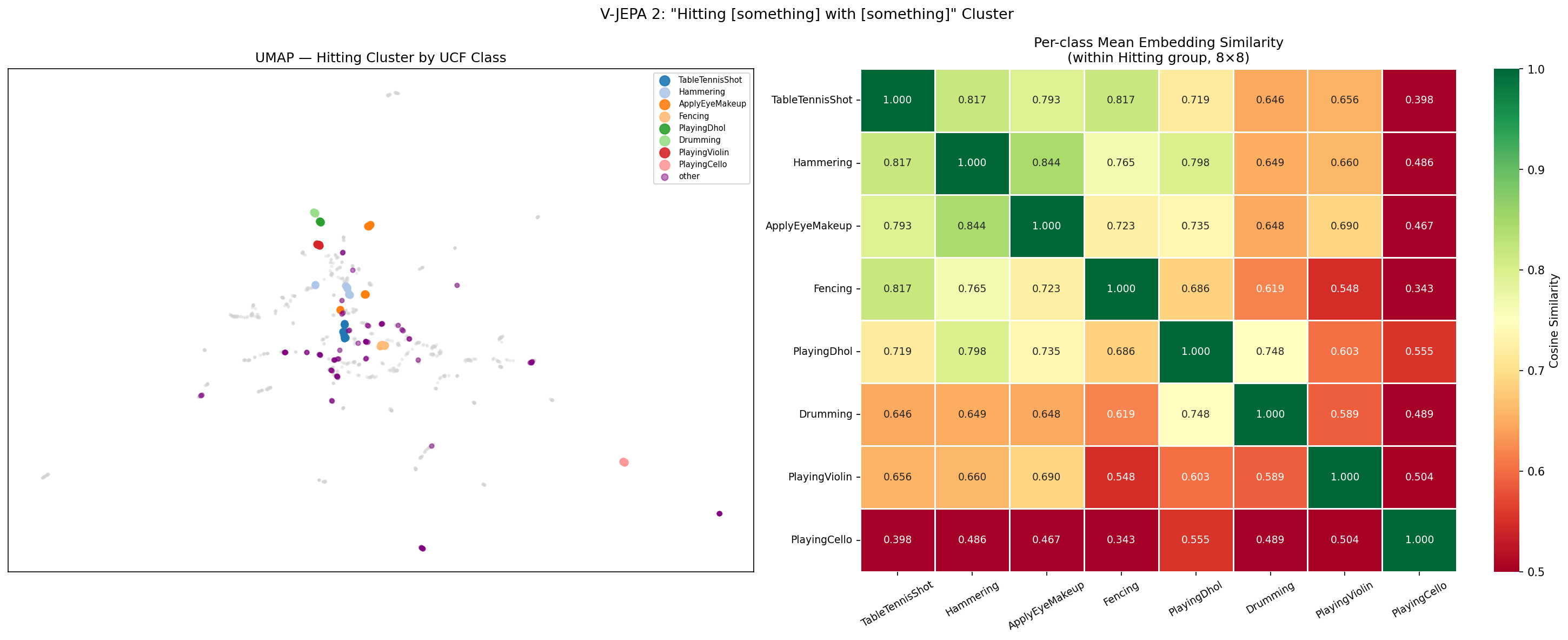
<p>“Hitting [something] with [something]” absorbed 33 different UCF
classes. Testing whether this is a genuine physics cluster:</p>

<table>
  <thead>
    <tr>
      <th>Metric</th>
      <th>Value</th>
    </tr>
  </thead>
  <tbody>
    <tr>
      <td>Within-group cosine similarity</td>
      <td>0.61</td>
    </tr>
    <tr>
      <td>Global same-class baseline</td>
      <td>0.93</td>
    </tr>
  </tbody>
</table>

<p>The 0.32 gap below baseline confirms spurious absorption. The label
functions as a miscellaneous bin for any repetitive contact motion.
TableTennisShot, ApplyEyeMakeup, and Hammering share it not because
their underlying physics is similar but because none fit cleanly into
any other SSv2 category.</p>

<p><img src="/assets/images/vjepa2_hitting_cluster.png" alt="Hitting cluster analysis" />
<em>Left: UMAP showing all 33 UCF classes predicted as “Hitting”, colored by UCF class. The spread confirms they are not a tight geometric cluster. Right: 8×8 pairwise cosine similarity heatmap for the top 8 UCF classes in the hitting group. TableTennisShot and Hammering are geometrically distant despite sharing the same SSv2 label.</em></p>

<h3 id="hypothesis-testing-what-drives-behavior-categories">Hypothesis Testing: What Drives Behavior Categories?</h3>

<p>Three hypotheses tested using embedding-derived proxies:</p>

<table>
  <thead>
    <tr>
      <th>Hypothesis</th>
      <th>Proxy</th>
      <th>Pearson r</th>
      <th>p-value</th>
      <th>Verdict</th>
    </tr>
  </thead>
  <tbody>
    <tr>
      <td>A: Temporal dynamics</td>
      <td>Intra-class embedding variance</td>
      <td>-0.20</td>
      <td>0.043</td>
      <td>PARTIALLY SUPPORTED</td>
    </tr>
    <tr>
      <td>B: Spatial scale</td>
      <td>Distance from SSv2 distribution center</td>
      <td>+0.02</td>
      <td>0.87</td>
      <td>REJECTED</td>
    </tr>
    <tr>
      <td>C: Cluster tightness</td>
      <td>Within-class cosine similarity</td>
      <td>+0.15</td>
      <td>0.13</td>
      <td>REJECTED</td>
    </tr>
  </tbody>
</table>

<p>Hypothesis A is the strongest signal: periodic, repeatable actions
embed more consistently across video instances and tend to receive
higher confidence predictions. But r²≈0.04 means it explains only
4% of variance. Hypotheses B and C are not supported.</p>

<p>The geometry of where a class sits in embedding space, and how
tightly it clusters, does not reliably predict whether the SSv2
head will be confident. Something more nuanced, likely the degree
of overlap between the action’s motion vocabulary and SSv2’s physics
primitive vocabulary, is the actual driver, but that is not
directly measurable from frozen embeddings alone.</p>

<h3 id="the-tight-cluster-paradox">The Tight Cluster Paradox</h3>

<p>21 LOW_CONF_SCATTERED classes have above-median within-class cosine
similarity. Their embeddings are geometrically tight: the backbone
encodes them consistently, yet the SSv2 head produces low-confidence
scattered predictions. These 21 classes are the clearest pre-linear-probe
evidence that the backbone has encoded structure the SSv2 head lacks
vocabulary to express.</p>

<hr />

<h2 id="phase-4-linear-probe">Phase 4: Linear Probe</h2>

<p>A logistic regression classifier (L2 regularised, <code class="language-plaintext highlighter-rouge">lbfgs</code> solver,
stratified 5-fold cross-validation, StandardScaler fit on train folds
only) trained on the frozen (1059, 1024) embeddings with UCF-101 labels.</p>

<p><strong>Overall accuracy: 98.2% ± 1.0%</strong></p>

<table>
  <thead>
    <tr>
      <th>Behavior category</th>
      <th>Linear probe accuracy</th>
    </tr>
  </thead>
  <tbody>
    <tr>
      <td>HIGH_CONF_CONSISTENT</td>
      <td>~99%</td>
    </tr>
    <tr>
      <td>HIGH_CONF_INCONSISTENT</td>
      <td>~98%</td>
    </tr>
    <tr>
      <td>LOW_CONF_SCATTERED</td>
      <td>~97%</td>
    </tr>
  </tbody>
</table>

<p>All four blind-spot classes:</p>

<table>
  <thead>
    <tr>
      <th>Class</th>
      <th>SSv2 confidence</th>
      <th>Linear probe accuracy</th>
      <th>Delta</th>
    </tr>
  </thead>
  <tbody>
    <tr>
      <td>PoleVault</td>
      <td>0.168</td>
      <td>100%</td>
      <td>+83.2%</td>
    </tr>
    <tr>
      <td>WritingOnBoard</td>
      <td>0.189</td>
      <td>100%</td>
      <td>+81.1%</td>
    </tr>
    <tr>
      <td>SalsaSpin</td>
      <td>0.194</td>
      <td>100%</td>
      <td>+80.6%</td>
    </tr>
    <tr>
      <td>Surfing</td>
      <td>~0.20</td>
      <td>100%</td>
      <td>~+80%</td>
    </tr>
  </tbody>
</table>

<p>The tight cluster paradox resolution:</p>

<table>
  <thead>
    <tr>
      <th>Metric</th>
      <th>Value</th>
    </tr>
  </thead>
  <tbody>
    <tr>
      <td>Mean linear probe accuracy (21 scattered classes)</td>
      <td>99.5%</td>
    </tr>
    <tr>
      <td>Mean SSv2 confidence (same 21 classes)</td>
      <td>30.8%</td>
    </tr>
    <tr>
      <td>Delta</td>
      <td>+68.7%</td>
    </tr>
  </tbody>
</table>

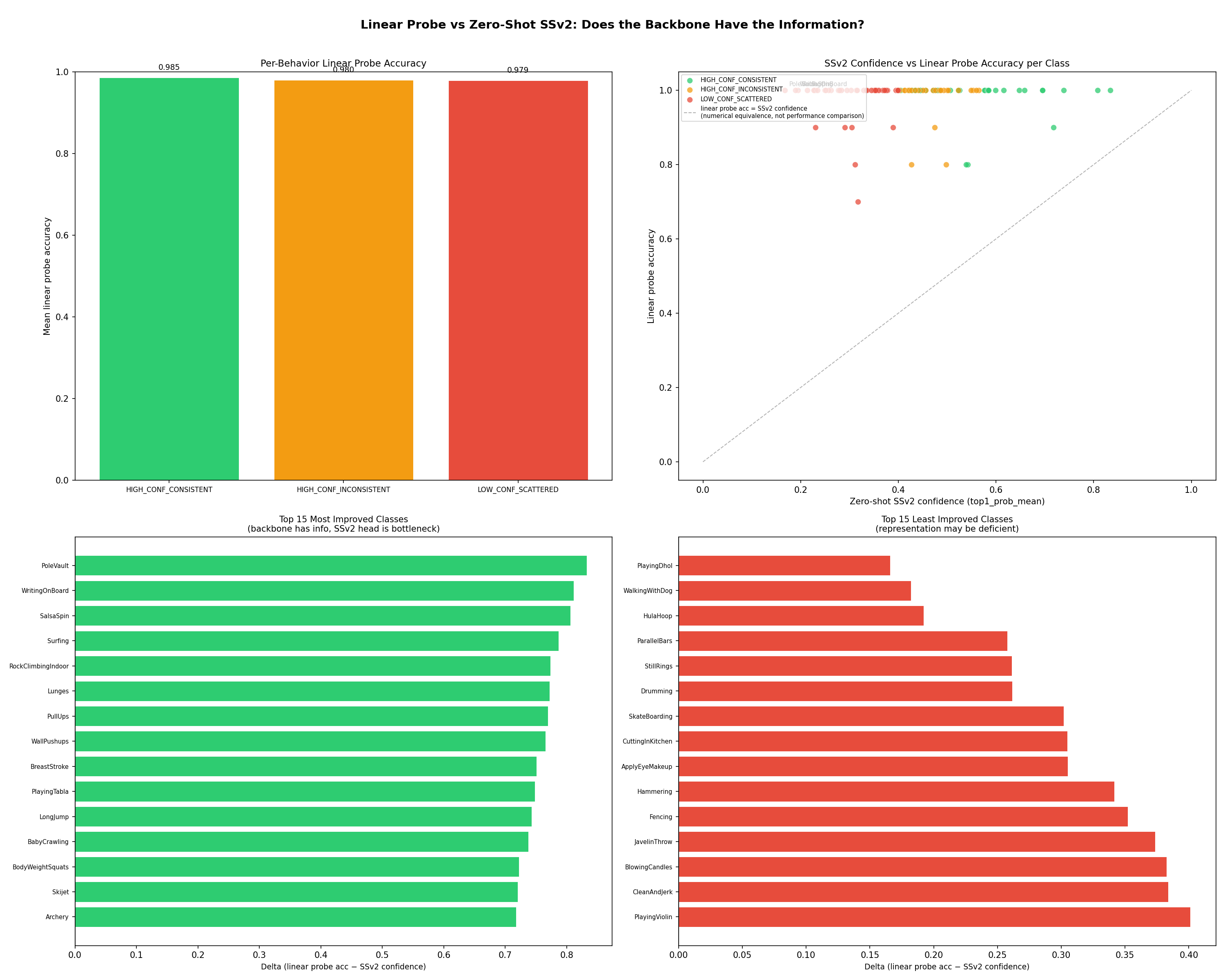
<p>There is no UCF-101 class where the backbone fails. The worst
performer is WalkingWithDog at 90%, the only class where the SSv2
head was already somewhat confident (0.718), leaving less room to
improve.</p>

<p><img src="/assets/images/vjepa2_linear_probe.png" alt="Linear probe results" />
<em>Top left: per-behavior accuracy with error bars. Top right: scatter of SSv2 confidence (x) vs linear probe accuracy (y) per class; points above the diagonal have more linearly separable embeddings than the SSv2 head’s confidence suggests. Bottom: top 15 most and least improved classes by delta.</em></p>

<hr />

<h2 id="conclusion">Conclusion</h2>

<p>The linear probe result closes the causal question the embedding
analysis raised. The backbone encodes all 101 UCF-101 action categories
at 98.2% linear separability. The SSv2 classification head, a
supervised component with a fixed 174-word vocabulary, cannot express
42% of what the backbone knows.</p>

<p>For practitioners adapting V-JEPA 2 to a new action domain: the
backbone is not the bottleneck. Replacing the SSv2 head with a linear
mapping trained on even a small labeled set from the target domain
is sufficient to recover near-ceiling accuracy. Full backbone
fine-tuning is unlikely to produce meaningful gains over head
replacement alone, at substantially higher cost.</p>

<p>This finding connects to a broader pattern in JEPA-style architectures.
In my earlier <a href="https://hellojais.github.io/machine-learning/world-models/research/2026/05/09/what-billiards-reveals-about-jepa.html">billiards study</a>,
the LeWM backbone encoded ball position at R²=0.988 from pure pixel
prediction, but the downstream planning component was the bottleneck.
The same separation appears here: self-supervised pre-training produces
representations that generalize well beyond the training distribution.
The supervised components built on top of them are the limiting factor.</p>

<hr />

<h2 id="limitations">Limitations</h2>

<ul>
  <li>~10 videos per class. Results are internally valid for relative
comparison across classes but not representative of large-sample
linear probe benchmarks.</li>
  <li>The linear probe uses the same embeddings as the analysis phases.
There is no fully held-out evaluation set.</li>
  <li>Single model (V-JEPA 2 ViT-L), single dataset (UCF-101). Generalization
to other architectures or datasets is not established here.</li>
</ul>

<hr />

<h2 id="whats-next">What’s Next</h2>

<ol>
  <li><strong>Kinetics-400</strong>: does the 98.2% linear probe result hold on a
larger, more diverse benchmark?</li>
  <li><strong>Head replacement vs LoRA</strong>: does fine-tuning the backbone improve
over a pure linear head swap, or is the backbone already at ceiling?</li>
  <li><strong>Optical flow for temporal dynamics</strong>: Hypothesis A was only
partially supported using embedding variance as a proxy. Direct
measurement of motion periodicity from optical flow would give a
cleaner test of whether temporal periodicity drives confidence.</li>
  <li><strong>Cross-architecture comparison</strong>: does a CLIP-based video model
show the same backbone/head dissociation, or is this specific to
JEPA-style predictive pre-training?</li>
  <li><strong>Few-shot head adaptation</strong>: how few labeled examples per class
does a linear head need to reach 95%+ on a new action domain?</li>
</ol>

<hr />

<h2 id="resources">Resources</h2>

<table>
  <thead>
    <tr>
      <th>Resource</th>
      <th>Link</th>
    </tr>
  </thead>
  <tbody>
    <tr>
      <td>💻 Code</td>
      <td><a href="https://github.com/hellojais/vjepa2-live">hellojais/vjepa2-live</a></td>
    </tr>
    <tr>
      <td>📊 Full Report</td>
      <td><a href="https://github.com/hellojais/vjepa2-live/blob/main/results/vjepa2_live_report.html">vjepa2_live_report.html</a></td>
    </tr>
    <tr>
      <td>🤖 Model</td>
      <td><a href="https://huggingface.co/qubvel-hf/vjepa2-vitl-fpc16-256-ssv2">qubvel-hf/vjepa2-vitl-fpc16-256-ssv2</a></td>
    </tr>
    <tr>
      <td>📁 Dataset</td>
      <td><a href="https://www.crcv.ucf.edu/data/UCF101.php">UCF-101</a></td>
    </tr>
  </tbody>
</table>

<hr />

<p><em>All code from this project is released under MIT license.</em></p>]]></content><author><name>Santosh Jaiswal</name></author><category term="machine-learning" /><category term="world-models" /><category term="representation-learning" /><summary type="html"><![CDATA[I ran V-JEPA 2 frozen on 1,059 UCF-101 videos it was never trained on. A linear probe on the frozen backbone hit 98.2%. The SSv2 classification head fails on 42% of classes. The representations are not the problem.]]></summary></entry><entry><title type="html">What Billiards Reveals About JEPA: Strong Physics Representations, a Precise Planning Boundary</title><link href="https://hellojais.github.io/machine-learning/world-models/research/2026/05/09/what-billiards-reveals-about-jepa.html" rel="alternate" type="text/html" title="What Billiards Reveals About JEPA: Strong Physics Representations, a Precise Planning Boundary" /><published>2026-05-09T00:00:00+00:00</published><updated>2026-05-09T00:00:00+00:00</updated><id>https://hellojais.github.io/machine-learning/world-models/research/2026/05/09/what-billiards-reveals-about-jepa</id><content type="html" xml:base="https://hellojais.github.io/machine-learning/world-models/research/2026/05/09/what-billiards-reveals-about-jepa.html"><![CDATA[<blockquote>
  <p><strong>Author:</strong> Santosh Jaiswal (<a href="https://github.com/hellojais">@hellojais</a>)<br />
<strong>Code:</strong> <a href="https://github.com/hellojais/le-wm">hellojais/le-wm</a>, a fork of <a href="https://github.com/lucas-maes/le-wm">lucas-maes/le-wm</a><br />
<strong>Dataset:</strong> <a href="https://huggingface.co/datasets/hellojais/billiards-worldmodel">hellojais/billiards-worldmodel</a><br />
<strong>Model:</strong> <a href="https://huggingface.co/hellojais/lewm-billiards">hellojais/lewm-billiards</a><br />
<strong>Game Code:</strong> <a href="https://github.com/hellojais/billiards-worldmodel">hellojais/billiards-worldmodel</a></p>
</blockquote>

<hr />

<h2 id="tldr">TL;DR</h2>

<p>I applied LeWM, a recently published JEPA-based world model, to 2D billiards, a domain nobody had tested it on. The model learned ball position excellently (R²=0.988) but velocity poorly (R²=0.33). Pure imagination-based planning failed because billiards is decided in a single collision frame that requires precise velocity simulation. A state-based hybrid approach succeeded on novel combinations never seen during training. These findings align with and concretely explain the Two-Room boundary condition described in the original LeWM paper: low visual complexity environments expose a specific limitation where JEPA’s isotropic Gaussian prior produces a latent space that is stable but insufficiently structured for goal-directed planning. A follow-up investigation identified a second failure mode (representational eviction under frame stacking) and an architectural fix (auxiliary state supervision) that recovers position R²=0.999 and velocity R²=0.947. The Update section below covers these results.</p>

<hr />

<h2 id="the-idea">The Idea</h2>

<p>A child watches billiards for the first time. Nobody explains angles, momentum, or collision physics. They just watch. Game after game, they build intuition: hit here, the ball goes there. After enough games, they can close their eyes and imagine what will happen before the shot is taken.</p>

<p>This is the core idea behind <strong>JEPA</strong> (Joint Embedding Predictive Architecture), proposed by Yann LeCun: instead of learning to reconstruct pixels, learn to predict what will happen next in a compressed latent space. It is a machine that learns by imagining.</p>

<p><a href="https://arxiv.org/abs/2603.19312">LeWM (Le World Model)</a>, published by Lucas Maes, Quentin Leroux, Gauthier Gidel, and Glen Berseth at Mila/McGill (2025), is the first JEPA that trains stably end-to-end from raw pixels using only two loss terms: a next-embedding prediction loss and SIGReg (Sketched-Isotropic-Gaussian Regularizer), which prevents representation collapse by enforcing an isotropic Gaussian distribution in latent space. This reduces tunable loss hyperparameters from six or seven (as in PLDM or VICReg) to just one (λ), while enabling planning up to 48× faster than foundation-model-based world models.</p>

<p>It has been demonstrated on Push-T (block manipulation), Reacher (robotic arm), Cube (3D pick-and-place), and Two-Room (navigation). Nobody had tried it on billiards. So I did.</p>

<hr />

<h2 id="push-t-vs-billiards-two-very-different-worlds">Push-T vs Billiards: Two Very Different Worlds</h2>

<p>Before diving into the experiments, it is worth understanding why Push-T works well for LeWM and billiards is a fundamentally harder test.</p>

<p><strong>Push-T is a quasi-static environment.</strong> The T-block moves incrementally in response to small ball pushes. Each step produces a small, smooth change in the scene. Planning horizons can be short because incremental corrective actions compensate for minor prediction drift. The spatial goals (block at position X, angle Y) are visually distinctive: a T-block rotated 30° looks clearly different from one rotated 200°, giving the latent space meaningful geometric structure to navigate.</p>

<p><strong>Billiards is a hostile environment.</strong> The key event, collision, is a sharp physical non-linearity compressed into a single frame. Ball velocity can change from near-zero to high-speed in one timestep. Planning requires long horizons and microscopic timing precision. And the visual diversity is low: two balls on a green background don’t vary dramatically frame-to-frame, leaving little signal for the encoder to organize the latent space around task-relevant structure.</p>

<p>The paper itself notes an interesting phenomenon in Push-T: trajectories exhibit emergent <strong>latent path straightening</strong>: consecutive latent velocity vectors become increasingly aligned, a property typically observed in biological vision systems, arising here without explicit temporal regularization. This straightening is beneficial for quasi-static tasks where smooth transitions dominate. In billiards, that same smoothing tendency becomes a liability: the predictor’s bias toward smooth transitions works against accurately modeling the sharp, instantaneous velocity change of a collision.</p>

<hr />

<h2 id="what-i-built">What I Built</h2>

<h3 id="the-game">The Game</h3>

<p>I built a 2D billiards environment in Python/Pygame: a 512×512 board with a white cue ball, a red target ball, and four corner pockets. A scripted expert agent uses the <strong>ghost-ball technique</strong> to aim:</p>

\[G = T - \hat{u}_{PT} \cdot 2R\]

<p>where \(T\) is the target ball position, \(\hat{u}_{PT}\) is the unit vector from pocket to target, and \(R\) is the ball radius. The agent computes the ideal contact point and applies an impulse, with small Gaussian noise for episode variety.</p>

<h3 id="the-dataset">The Dataset</h3>

<p>I recorded 4,000 instrumented episodes, not just video, but pixels, actions, and ground-truth game state saved together at every timestep:</p>

<table>
  <thead>
    <tr>
      <th>Key</th>
      <th>Shape</th>
      <th>Description</th>
    </tr>
  </thead>
  <tbody>
    <tr>
      <td><code class="language-plaintext highlighter-rouge">pixels</code></td>
      <td>(971321, 96, 96, 3)</td>
      <td>RGB frames</td>
    </tr>
    <tr>
      <td><code class="language-plaintext highlighter-rouge">action</code></td>
      <td>(971321, 2)</td>
      <td>(dx, dy) impulse applied to cue ball</td>
    </tr>
    <tr>
      <td><code class="language-plaintext highlighter-rouge">state</code></td>
      <td>(971321, 10)</td>
      <td>Full state vector (see below)</td>
    </tr>
    <tr>
      <td><code class="language-plaintext highlighter-rouge">ep_len</code></td>
      <td>(4000,)</td>
      <td>Frames per episode</td>
    </tr>
    <tr>
      <td><code class="language-plaintext highlighter-rouge">ep_offset</code></td>
      <td>(4000,)</td>
      <td>Start frame index per episode</td>
    </tr>
  </tbody>
</table>

<p>The state vector encodes 10 values: cue ball position (2), cue ball velocity (2), target ball position (2), target ball velocity (2), and nearest pocket position (2). While the meaningful degrees of freedom are essentially 4 numbers (two ball positions), storing velocities and pocket position gives richer supervision signal during probing experiments.</p>

<p><strong>Total: 971,321 frames, 368MB compressed (LZ4), ~56% episode success rate.</strong></p>

<p>The 56% success rate is intentional: failed episodes (where the agent ran out of steps before potting the ball) still contain valid physics signal. The model sees the ball moving, decelerating due to friction, and bouncing off walls regardless of outcome. Including failures makes the training distribution richer, not noisier.</p>

<p>This flat HDF5 format exactly matches the LeWM Push-T dataset structure, a deliberate choice to make the training pipeline a drop-in replacement.</p>

<h3 id="training-on-apple-silicon">Training on Apple Silicon</h3>

<p>I trained on an Apple M5 Max (128GB unified memory) using PyTorch’s MPS backend, with no CUDA and no cloud GPU. The stable-worldmodel library needed three fixes for MPS compatibility:</p>

<ol>
  <li><code class="language-plaintext highlighter-rouge">device='cuda'</code> hardcoded in the SIGReg loss → <code class="language-plaintext highlighter-rouge">device=proj.device</code></li>
  <li><code class="language-plaintext highlighter-rouge">pin_memory=True</code> in DataLoader → <code class="language-plaintext highlighter-rouge">False</code> (MPS doesn’t support pinned memory)</li>
  <li><code class="language-plaintext highlighter-rouge">num_workers=6</code> → <code class="language-plaintext highlighter-rouge">0</code> (MPS can’t share tensor storage across workers)</li>
</ol>

<p>These fixes are documented in <a href="https://github.com/hellojais/le-wm/blob/main/SETUP_NOTES.md">SETUP_NOTES.md</a> for anyone running LeWM on Apple Silicon.</p>

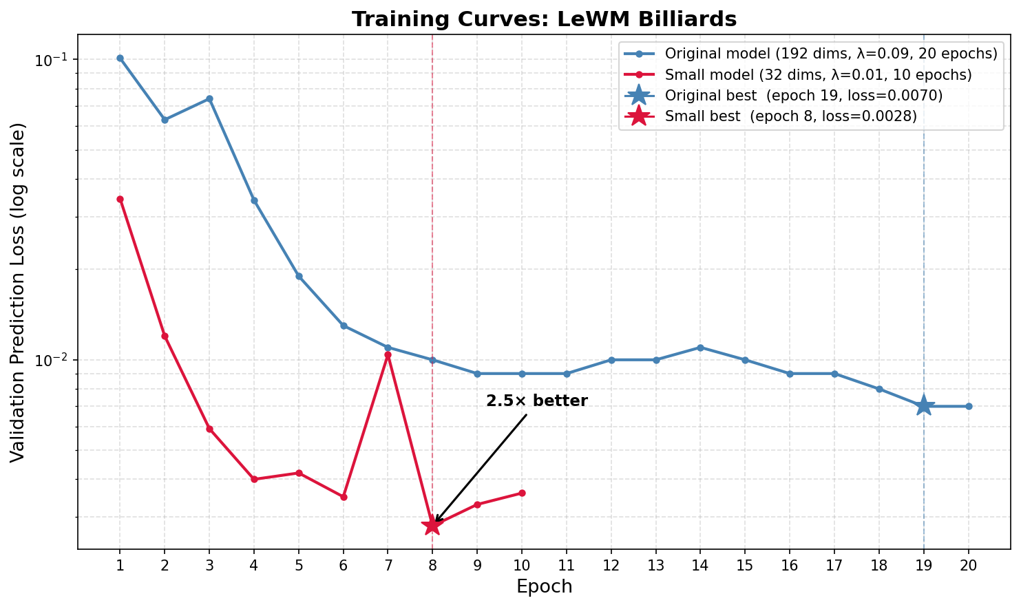
<p>LeWM’s efficient two-term objective (only one key hyperparameter λ, with an O(log n) bisection search for optimal regularization) made it straightforward to explore different configurations:</p>

<table>
  <thead>
    <tr>
      <th>Model</th>
      <th>embed_dim</th>
      <th>λ (SIGReg)</th>
      <th>Epochs</th>
      <th>Best val/pred_loss</th>
    </tr>
  </thead>
  <tbody>
    <tr>
      <td>Original</td>
      <td>192</td>
      <td>0.09</td>
      <td>20</td>
      <td>0.00737</td>
    </tr>
    <tr>
      <td>Small</td>
      <td>32</td>
      <td>0.01</td>
      <td>10</td>
      <td>0.00280</td>
    </tr>
  </tbody>
</table>

<p>Training time: ~20 hours for the original, ~10 hours for the small model, both on a single M5 Max.</p>

<p><img src="/assets/images/training_curves.png" alt="Training Curves" />
<em>Training curves for both models. The small model (32 dims, λ=0.01) achieves 2.6× better prediction accuracy in half the epochs.</em></p>

<hr />

<h2 id="the-planning-experiments">The Planning Experiments</h2>

<p>LeWM plans using <strong>CEM (Cross-Entropy Method)</strong>: sample thousands of action sequences, simulate them in the model’s imagination in embedding space (never touching the real environment), keep the best candidates, repeat. The cost function measures how close the imagined final embedding is to the goal embedding.</p>

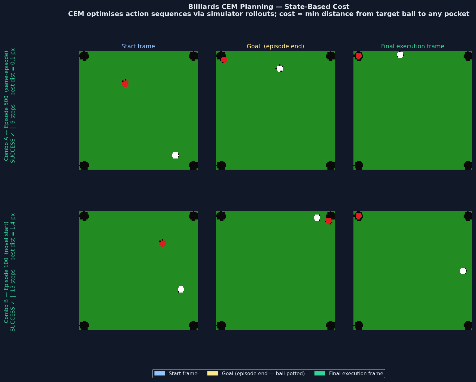
<p>I ran four systematic experiments with two goal combinations:</p>
<ul>
  <li><strong>Combo A:</strong> Same episode, start and goal from episode 500</li>
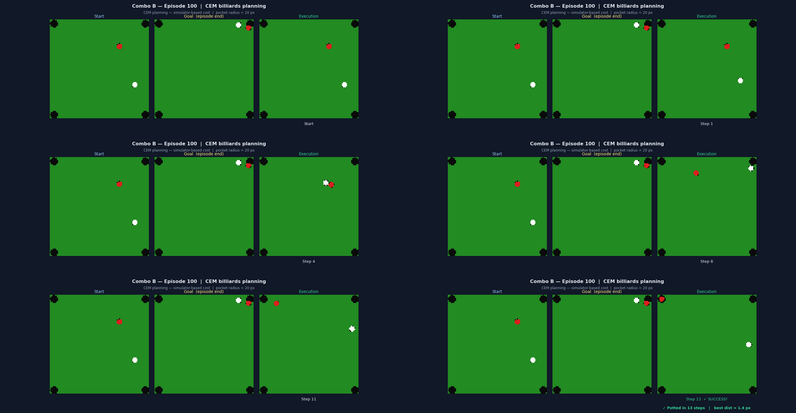
  <li><strong>Combo B:</strong> Novel cross-episode, start from episode 100, goal from episode 3,000 (never seen together during training)</li>
</ul>

<hr />

<h3 id="experiment-1-pure-jepa-embedding-cem-192-dims">Experiment 1: Pure JEPA Embedding CEM (192 dims)</h3>

<p><strong>Cost function:</strong> L2 distance between predicted final embedding and goal embedding.</p>

<p><strong>Result: ⚠️ No useful gradient signal</strong></p>

<p>The diagnosis: all embeddings sat roughly 20 L2 units apart from each other, whether scenes were similar or completely different. The embedding space was a uniform shell.</p>

<div class="language-plaintext highlighter-rouge"><div class="highlight"><pre class="highlight"><code>Mean pairwise distance:  19.38
Std pairwise distance:    1.56  ← too uniform
Min pairwise distance:   10.16
</code></pre></div></div>

<p>CEM had no hill to climb. Every action sequence looked equally far from the goal, so it could not tell a good shot from a bad one.</p>

<hr />

<h3 id="experiment-2-reduced-dimensions-32-dims-λ001">Experiment 2: Reduced Dimensions (32 dims, λ=0.01)</h3>

<p><strong>Hypothesis:</strong> Reducing embed_dim forces more aggressive compression. Lower SIGReg weight gives the model more freedom to cluster similar scenes together rather than forcing everything onto a uniform Gaussian shell.</p>

<p><strong>Result: ⚠️ Better prediction, same planning problem</strong></p>

<p>The prediction accuracy improved dramatically:</p>

<div class="language-plaintext highlighter-rouge"><div class="highlight"><pre class="highlight"><code>Prediction accuracy (pred→real L2):
  Original model: 0.946
  Small model:    0.111  ← 8.5× better
</code></pre></div></div>

<p>The embedding space became less uniform:</p>

<div class="language-plaintext highlighter-rouge"><div class="highlight"><pre class="highlight"><code>Min pairwise distance: 10.16 → 0.89  ← similar frames now cluster
CV (std/mean):          0.081 → 0.121 ← more varied
</code></pre></div></div>

<p>But planning still failed. Better prediction and less uniform embeddings are necessary but not sufficient for JEPA planning. The embedding space needs not just variation but <em>structured</em> variation: where the direction toward the goal corresponds to a meaningful gradient in the cost landscape.</p>

<hr />

<h3 id="experiment-3-probe-based-cem">Experiment 3: Probe-Based CEM</h3>

<p><strong>Hypothesis:</strong> Maybe the embedding space contains the right information but L2 distance is not the right way to access it. Train a small MLP to decode state from embeddings, use that as the cost function.</p>

<p><strong>Probe results:</strong></p>

<table>
  <thead>
    <tr>
      <th>Quantity</th>
      <th>R²</th>
    </tr>
  </thead>
  <tbody>
    <tr>
      <td>Target ball x</td>
      <td>0.988 ✅</td>
    </tr>
    <tr>
      <td>Target ball y</td>
      <td>0.976 ✅</td>
    </tr>
    <tr>
      <td>Nearest pocket x</td>
      <td>0.981 ✅</td>
    </tr>
    <tr>
      <td>Cue ball x</td>
      <td>0.854 ✅</td>
    </tr>
    <tr>
      <td>Target ball vx</td>
      <td>0.337 ⚠️</td>
    </tr>
    <tr>
      <td>Target ball vy</td>
      <td>0.371 ⚠️</td>
    </tr>
  </tbody>
</table>

<p>The model knew exactly where the ball was. But it barely knew how fast it was moving.</p>

<p>These probe results parallel the Push-T findings in the original paper: agent location (r=0.974) and block location (r=0.986) are encoded with similarly high fidelity. The difference is that Push-T planning doesn’t require velocity: incremental corrective actions compensate for any drift. Billiards planning lives or dies by velocity at the moment of collision.</p>

<p><strong>Result: ⚠️ Still failed</strong></p>

<p>Even with a near-perfect position cost function, CEM could not find action sequences that led to a potted ball. The bottleneck was the dynamics predictor itself. Prediction error per step (0.111 L2) was larger than the actual ball motion during collision events, meaning multi-step imagined trajectories diverged immediately after contact. This is the autoregressive error accumulation problem the paper warns about: small errors compound across open-loop CEM rollouts, causing the imagined trajectory to diverge from physical ground truth.</p>

<hr />

<h3 id="experiment-4-state-based-hybrid-cem">Experiment 4: State-Based Hybrid CEM</h3>

<p><strong>Hypothesis:</strong> If the embedding-distance cost has no gradient, replace it with a cost that does: distance of target ball to nearest pocket, measured in the real simulator.</p>

<p><strong>Important clarification:</strong> The world model is still doing the heavy lifting here. The predictor still imagines future trajectories in embedding space. What changed is only the <em>judge</em>: instead of asking “is this imagined embedding close to the goal embedding?”, we ask “when we execute this planned action sequence in the real simulator, does the ball get close to a pocket?” The judging is done by the simulator because the embedding space lacks the structured geometry needed for L2-based navigation.</p>

<p><strong>Result: ✅ SUCCESS on both combos</strong></p>

<table>
  <thead>
    <tr>
      <th>Combo</th>
      <th>Result</th>
      <th>Steps</th>
    </tr>
  </thead>
  <tbody>
    <tr>
      <td>A (same episode)</td>
      <td>✅ Potted</td>
      <td>9 steps</td>
    </tr>
    <tr>
      <td>B (novel cross-episode)</td>
      <td>✅ Potted</td>
      <td>13 steps</td>
    </tr>
  </tbody>
</table>

<p><img src="/assets/images/planning_results.png" alt="Planning Results" />
<em>Start frame, goal frame, and execution result for both combos.</em></p>

<p><img src="/assets/images/combo_b_planning.gif" alt="Combo B Planning" />
<em>Novel cross-episode planning: start from episode 100, goal from episode 3,000. The model generalizes: it did not memorize this combination, it had to reason about billiards physics it learned.</em></p>

<p>Crucially, Combo B, a start/goal combination that never appeared in training, succeeded. This confirms the model learned generalizable billiards physics, not episode memorization. The planner naturally converged to strong impulse shots (9-12 env units), exactly what billiards requires. When embedding-based CEM was used, it stayed at 1-4 units because the embedding landscape gave no gradient toward stronger shots.</p>

<hr />

<h2 id="the-root-cause-velocity-encoding-gap">The Root Cause: Velocity Encoding Gap</h2>

<p>The probe results point to a specific architectural limitation.</p>

<p>The ViT encoder processes <strong>each frame independently</strong>. Velocity is only implicit, inferred from the difference between consecutive embeddings passed to the predictor. For a visually complex environment like Push-T, this implicit signal is rich enough. For billiards, where two balls on a green background barely vary from frame to frame, the signal is too weak.</p>

<div class="language-plaintext highlighter-rouge"><div class="highlight"><pre class="highlight"><code>Position:  R² = 0.988  ← encoder knows WHERE the ball is
Velocity:  R² = 0.33   ← encoder barely knows HOW FAST
</code></pre></div></div>

<p>Billiards planning is decided by velocity at the moment of collision: one frame, one instant. If the predictor cannot accurately simulate that moment, multi-step imagination drifts immediately after contact.</p>

<p>This aligns precisely with what the LeWM paper observed for Two-Room: <em>“low intrinsic dimensionality may hinder the Gaussian regularizer from producing a well-structured latent space.”</em> Billiards is an extreme case of this: the game state is fundamentally 4 numbers (two ball positions) yet we compress it into 32-192 dimensions, giving SIGReg too much room to spread representations uniformly rather than organizing them by task-relevant structure.</p>

<p>There is also a subtler mechanism at work. The emergent <strong>latent path straightening</strong> observed in Push-T (where trajectory vectors become increasingly aligned in latent space, a property of biological vision systems arising here without explicit regularization) is a property of smooth, quasi-static dynamics. In billiards, that same smoothing tendency is a liability: the predictor’s bias toward gradual transitions works against modeling the sharp, instantaneous velocity change of a collision. The model imagines a gentler world than the one that actually exists at the moment of impact.</p>

<hr />

<h2 id="the-latent-space">The Latent Space</h2>

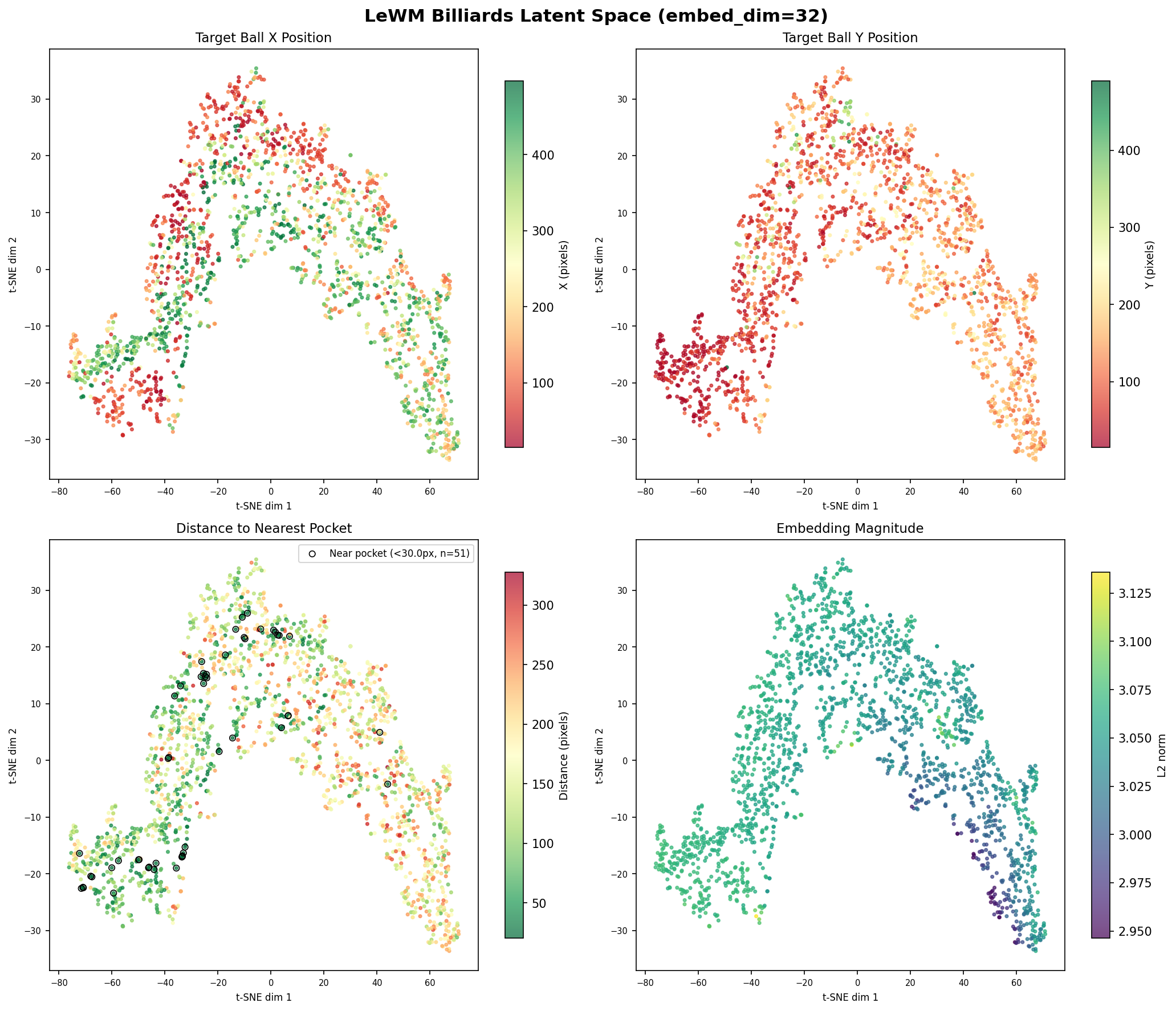
<p>Despite the planning limitations, the t-SNE visualization confirms the model learned meaningful structure:</p>

<p><img src="/assets/images/tsne_billiards.png" alt="t-SNE Latent Space" />
<em>t-SNE of 2,000 frame embeddings colored by: target ball X position (top-left), target ball Y position (top-right), distance to nearest pocket (bottom-left), embedding magnitude (bottom-right).</em></p>

<p>Regions of the embedding map correspond loosely to different table positions, confirming position is encoded. But near-pocket frames (black circles, bottom-left) are scattered across the entire map rather than clustering, visually confirming why CEM had no gradient to follow toward the goal.</p>

<p>The model also passes a stronger test: Violation-of-Expectation (VoE). The paper shows LeWM assigns significantly higher surprise (MSE spikes) to physical violations like teleportation than to visual perturbations like color changes (paired t-test, p&lt;0.01). The model genuinely understands physical continuity, not just pattern-matching pixels. The gap between understanding physics and accurately predicting the precise outcome of a high-velocity collision is the specific limitation we have isolated.</p>

<hr />

<h2 id="what-this-means">What This Means</h2>

<p>The complete picture:</p>

<table>
  <thead>
    <tr>
      <th>What worked</th>
      <th>What did not</th>
    </tr>
  </thead>
  <tbody>
    <tr>
      <td>Training stability (SIGReg) ✅</td>
      <td>Embedding-distance planning ⚠️</td>
    </tr>
    <tr>
      <td>Position encoding (R²=0.988) ✅</td>
      <td>Velocity encoding (R²=0.33) ⚠️</td>
    </tr>
    <tr>
      <td>Generalizing to novel combinations ✅</td>
      <td>Collision mechanics simulation ⚠️</td>
    </tr>
    <tr>
      <td>Physical continuity understanding (VoE) ✅</td>
      <td>Pure JEPA imagination planning ⚠️</td>
    </tr>
    <tr>
      <td>State-based hybrid planning ✅</td>
      <td>Autoregressive error accumulation ⚠️</td>
    </tr>
  </tbody>
</table>

<p>This is not a failure of JEPA. The encoder learned rich physics representations, with position encoded at R²=0.988 after training purely from pixels and no explicit supervision. The limitation is specific and identifiable: in low visual complexity, high-precision physics environments, the embedding space needs additional structure for embedding-distance-based planning to work. The state-based hybrid approach succeeds, but the intellectually interesting challenge is making pure imagination-based planning work without the simulator. Subsequent experiments on the velocity encoding gap and an architectural fix are covered in the Update section below.</p>

<hr />

<h2 id="whats-next">What’s Next</h2>

<p>Three remaining directions (frame stacking and auxiliary supervision have since been tested; see Update section below):</p>

<p><strong>1. Contrastive objective for goal states</strong>
Explicitly train the model so that “ball near pocket” embeddings cluster together, distinct from “ball far from pocket.” This addresses the uniform shell problem at its root, giving CEM a real gradient to follow rather than patching around it.</p>

<p><strong>2. Hierarchical world modeling</strong>
Implement temporal hierarchies that decouple high-level strategic reasoning (pocket selection) from low-level motor control (precise cue strike). This would extend the effective planning horizon by separating what to do from how to do it precisely, particularly relevant for billiards where the strategic decision (which pocket) and the execution precision (exact impulse angle) operate on very different timescales.</p>

<p><strong>3. Inverse dynamics modeling</strong>
Learn action representations through inverse dynamics: inferring what action caused a transition rather than predicting forward from actions. This directly addresses the velocity encoding gap: instead of the encoder inferring velocity implicitly from pixel differences, the inverse dynamics model is explicitly trained to recover the action (impulse direction and magnitude) that produced a given state transition. For billiards, where the cue ball impulse determines everything about the subsequent collision, this gives the model a direct supervision signal for the physical quantity that matters most.</p>

<hr />

<h2 id="update-three-more-experiments">Update: Three More Experiments</h2>

<p>After publishing the original post, the velocity encoding gap pointed to two natural fixes: give the encoder explicit motion signal, and force it to preserve position. We ran three more experiments to test these hypotheses.</p>

<p><strong>Summary across all four model variants (192-dim CLS probe):</strong></p>

<table>
  <thead>
    <tr>
      <th>Model</th>
      <th>Key change</th>
      <th>val/pred_loss</th>
      <th>pos R²</th>
      <th>vel R²</th>
    </tr>
  </thead>
  <tbody>
    <tr>
      <td>Transformer baseline</td>
      <td>none</td>
      <td>0.0035</td>
      <td>≈0.983*</td>
      <td>≈0.178*</td>
    </tr>
    <tr>
      <td>Mamba predictor</td>
      <td>Stateful S6 predictor</td>
      <td>0.0034</td>
      <td>0.983†</td>
      <td>0.297†</td>
    </tr>
    <tr>
      <td>Frame stacking</td>
      <td>9-channel input</td>
      <td>0.00594</td>
      <td>0.446</td>
      <td>0.138</td>
    </tr>
    <tr>
      <td>AuxLoss full</td>
      <td>+ auxiliary state head</td>
      <td><strong>0.00105</strong></td>
      <td><strong>0.999</strong></td>
      <td><strong>0.947</strong></td>
    </tr>
  </tbody>
</table>

<p>*Estimated; 192-dim probe not run separately for this model.<br />
†32-dim probe values; 192-dim probe not run for Mamba.</p>

<p><strong>Mamba predictor: the bottleneck is the encoder, not the predictor.</strong> The original post speculated that the Transformer predictor’s fixed 3-frame context might be failing to accumulate velocity history. Replacing it with a Mamba (S6) predictor (which maintains persistent hidden state and can in principle integrate velocity over arbitrary histories) made no meaningful difference: velocity R² moved from 0.296 to 0.297, and prediction loss fell only 3.1%. Architecture is not the bottleneck. The problem sits upstream in what the encoder captures from a single frame.</p>

<p><strong>Frame stacking: explicit optical flow triggers representational eviction.</strong> Stacking three consecutive frames as 9 input channels makes pixel-level motion literally visible to the encoder’s first layer. Target ball velocity did improve, from R² ≈ 0.30 to R² ≈ 0.76 at the 32-dim level (extended probe). But at the 192-dim CLS level, position collapsed from R² = 0.983 to R² = 0.446 and overall velocity R² fell to 0.138, because the cue ball velocity signal was almost completely evicted (R² ≈ 0.06). The encoder made a rational optimisation choice: with optical flow available, velocity is more predictive of the next embedding than absolute position, so SIGReg’s fixed-capacity isotropic regularisation caused the model to trade spatial completeness for motion encoding. We call this <strong>representational eviction</strong>: JEPA’s single prediction objective cannot simultaneously optimise for next-state predictability (training signal) and goal-relevant spatial completeness (planning requirement). Both quantities are needed for planning; neither alone suffices.</p>

<p><strong>Auxiliary state supervision: full recovery and a 3.3× prediction gain.</strong> The fix is a lightweight <code class="language-plaintext highlighter-rouge">AuxStateHead</code> (LayerNorm(192) → Linear(192→10)) attached to the ViT CLS token during training, predicting all 10 ground-truth state dimensions with a small auxiliary loss (λ_aux = 0.1). The head is discarded at inference; its only role is to provide a gradient signal strong enough to counteract the regularisation pressure that caused eviction. At 192-dim, position R² recovered to 0.999 and velocity R² to 0.947. The combined model’s val/pred_loss of 0.00105 is <strong>3.3× lower than the Transformer baseline</strong>, demonstrating that richer representations actually aid prediction rather than conflicting with it. The mild tension with JEPA’s self-supervised ethos is analogous to SIGReg itself, which also adds a supervised geometric constraint to the embedding space.</p>

<p>The encoder bottleneck is resolved, but planning still fails. In subsequent experiments, CEM with the fixed encoder and a pocket-proximity cost achieved at best 28% progress (best seed: 147.5px vs. 213.9px start distance); a state-based planner using ground-truth physics succeeded 5/5 on novel cross-episode combinations. Fixing the encoder is necessary but not sufficient: predictor rollout accuracy at collision timesteps is the second, still-open bottleneck.</p>

<p>For complete technical details, per-dimension R² breakdowns, and extended probe diagnostics, see <a href="https://github.com/hellojais/le-wm/blob/main/FINDINGS.md">FINDINGS.md</a>.</p>

<hr />

<h2 id="resources">Resources</h2>

<table>
  <thead>
    <tr>
      <th>Resource</th>
      <th>Link</th>
    </tr>
  </thead>
  <tbody>
    <tr>
      <td>📊 Dataset</td>
      <td><a href="https://huggingface.co/datasets/hellojais/billiards-worldmodel">hellojais/billiards-worldmodel</a></td>
    </tr>
    <tr>
      <td>🤖 Model</td>
      <td><a href="https://huggingface.co/hellojais/lewm-billiards">hellojais/lewm-billiards</a></td>
    </tr>
    <tr>
      <td>💻 Code</td>
      <td><a href="https://github.com/hellojais/le-wm">hellojais/le-wm</a></td>
    </tr>
    <tr>
      <td>🎮 Game Code</td>
      <td><a href="https://github.com/hellojais/billiards-worldmodel">hellojais/billiards-worldmodel</a></td>
    </tr>
    <tr>
      <td>📄 Findings</td>
      <td><a href="https://github.com/hellojais/le-wm/blob/main/FINDINGS.md">FINDINGS.md</a></td>
    </tr>
    <tr>
      <td>🛠️ Setup (M5 Max)</td>
      <td><a href="https://github.com/hellojais/le-wm/blob/main/SETUP_NOTES.md">SETUP_NOTES.md</a></td>
    </tr>
  </tbody>
</table>

<hr />

<h2 id="credits">Credits</h2>

<p>Original LeWM architecture and paper:</p>

<blockquote>
  <p>Lucas Maes, Quentin Leroux, Gauthier Gidel, Glen Berseth<br />
<em>“LeWorldModel: Stable End-to-End Joint-Embedding Predictive Architecture from Pixels”</em><br />
Mila / McGill University (2025)<br />
<a href="https://arxiv.org/abs/2603.19312">arXiv:2603.19312</a> | <a href="https://github.com/lucas-maes/le-wm">GitHub</a></p>
</blockquote>

<p>This work builds directly on their codebase and training infrastructure. All credit for the LeWM architecture, SIGReg regularizer, and CEM planning framework belongs to the original authors.</p>

<hr />

<p><em>All code, data, and trained models from this project are released under MIT license.</em></p>]]></content><author><name>Santosh Jaiswal</name></author><category term="machine-learning" /><category term="world-models" /><category term="research" /><category term="jepa" /><category term="lewm" /><category term="billiards" /><category term="world-model" /><category term="apple-silicon" /><category term="pytorch" /><summary type="html"><![CDATA[I applied LeWM to 2D billiards and discovered two sequential bottlenecks for JEPA-based planning: a representational eviction failure mode under frame stacking, and an architectural fix (auxiliary state supervision) that fully recovers both position and velocity encoding. Seven experiments, two findings.]]></summary><media:thumbnail xmlns:media="http://search.yahoo.com/mrss/" url="https://hellojais.github.io/assets/images/combo_b_planning.gif" /><media:content medium="image" url="https://hellojais.github.io/assets/images/combo_b_planning.gif" xmlns:media="http://search.yahoo.com/mrss/" /></entry><entry><title type="html">Validating Google’s TurboQuant: 5x KV Cache Compression on the M5 Max</title><link href="https://hellojais.github.io/machine-learning/inference/local-ai/2026/04/14/validating-turboquant-on-m5-max.html" rel="alternate" type="text/html" title="Validating Google’s TurboQuant: 5x KV Cache Compression on the M5 Max" /><published>2026-04-14T00:00:00+00:00</published><updated>2026-04-14T00:00:00+00:00</updated><id>https://hellojais.github.io/machine-learning/inference/local-ai/2026/04/14/validating-turboquant-on-m5-max</id><content type="html" xml:base="https://hellojais.github.io/machine-learning/inference/local-ai/2026/04/14/validating-turboquant-on-m5-max.html"><![CDATA[<blockquote>
  <p><strong>Author:</strong> Santosh Jaiswal (<a href="https://github.com/hellojais">@hellojais</a>) <br />
<strong>Paper:</strong> <a href="https://lnkd.in/gukvqcQs">TurboQuant (ICLR 2026)</a> <br />
<strong>Library:</strong> <a href="https://lnkd.in/gXkdWeYp">mlx-optiq / mlx-vlm</a> by <a href="https://github.com/PrinceCuber">Prince Canuma</a> and contributors</p>
</blockquote>

<hr />

<h2 id="tldr">TL;DR</h2>

<p>I validated Google Research and DeepMind’s TurboQuant (ICLR 2026) on an Apple M5 Max with 128GB unified memory. Running Qwen-7B at a 32k context window, KV cache RAM dropped from <strong>4.2 GB to 0.85 GB</strong> (a <strong>5x reduction</strong>), with <strong>100% Needle-in-a-Haystack retrieval accuracy</strong> preserved. TurboQuant is data-oblivious: no retraining, no model modification, works with any Transformer. For local and agentic workflows, that is a significant practical result.</p>

<hr />

<h2 id="the-question">The Question</h2>

<p>I recently picked up a MacBook Pro M5 Max (128GB unified memory, 40-core GPU) with one question in mind: how far can you push local AI inference before you hit the memory wall?</p>

<p>The KV cache is usually where that wall appears. For long-context tasks (32k tokens and beyond), the cache alone can consume several gigabytes of RAM, grow linearly with context length, and either crash your run or force you onto cloud hardware. This is especially painful for agentic workflows that maintain long tool-use chains across many turns.</p>

<p>Perfect timing: just days after I got the machine, Google Research and DeepMind dropped <strong>TurboQuant</strong> at ICLR 2026. It targets exactly this bottleneck.</p>

<hr />

<h2 id="what-turboquant-does">What TurboQuant Does</h2>

<p>KV cache quantization is not new, but most approaches have a catch: they require calibration data, fine-tuning, or model-specific modification. TurboQuant is <strong>data-oblivious</strong>: it compresses the KV cache on the fly, at inference time, with no access to training data and no changes to model weights.</p>

<p>The mechanism in brief:</p>

<ol>
  <li><strong>Rotate the data</strong> into a distribution that is more predictable (lower effective entropy per dimension).</li>
  <li><strong>Quantize aggressively</strong> to 3.5-bit in my experiment.</li>
  <li><strong>Add a 1-bit correction path</strong> that handles the residual rounding error from step 2.</li>
</ol>

<p>The rotation step is the key insight. Raw key/value tensors have high variance in a small number of dimensions and low variance in most others, a structure that conventional uniform quantization handles poorly. After rotation, the variance is spread more evenly, and a fixed low-bit quantizer wastes far fewer bits on noise.</p>

<p>The math is non-trivial (the paper is worth a read; I used NotebookLM to work through it), but the practical implication is clean: you get aggressive compression without a calibration pipeline.</p>

<hr />

<h2 id="the-setup">The Setup</h2>

<p><strong>Hardware:</strong> MacBook Pro M5 Max, 128GB unified memory, 40-core GPU
<strong>Model:</strong> Qwen-7B
<strong>Context window:</strong> 32,000 tokens
<strong>Quantization library:</strong> mlx-optiq (Apple Silicon implementation by Prince Canuma and contributors)</p>

<p>A big shout-out to the OSS community here. An mlx-optiq implementation landed almost immediately after the paper dropped, which made validation on Apple Silicon surprisingly straightforward.</p>

<p><strong>Baseline:</strong> Standard FP16 inference, 32k context, no KV cache compression.</p>

<p><strong>Test:</strong> Needle-in-a-Haystack: embed a specific fact inside a 32,000-token document, then ask the model to retrieve it. This is a standard long-context stress test: if KV cache compression degrades the representation of distant tokens, retrieval fails.</p>

<hr />

<h2 id="results">Results</h2>

<table>
  <thead>
    <tr>
      <th>Configuration</th>
      <th>KV Cache RAM</th>
      <th>Retrieval accuracy</th>
    </tr>
  </thead>
  <tbody>
    <tr>
      <td>FP16 baseline (no compression)</td>
      <td>4.2 GB</td>
      <td>100%</td>
    </tr>
    <tr>
      <td>TurboQuant 3.5-bit</td>
      <td>0.85 GB</td>
      <td>100%</td>
    </tr>
  </tbody>
</table>

<p><strong>RAM reduction: 4.2 GB → 0.85 GB (5x)</strong></p>

<p>The compression held up exactly where it needed to. The Needle was found instantly. Retrieval accuracy stayed at 100% despite the aggressive 3.5-bit quantization. No degradation on the task that matters most for long-context agentic work: remembering what was said earlier.</p>

<hr />

<h2 id="why-this-matters-for-local-agentic-workflows">Why This Matters for Local Agentic Workflows</h2>

<p>The standard objection to running serious AI locally is memory. A long tool-use chain (where the model maintains context across dozens of function calls, intermediate results, and user turns) can easily push 20k-50k tokens of context. At FP16, that KV cache fills RAM fast.</p>

<p>5x compression changes that calculus. What previously required 20 GB of KV cache memory now fits in 4 GB. On a machine with 128GB unified memory, this means you can run significantly longer chains, larger models, or multiple concurrent sessions before hitting the wall.</p>

<p>More broadly: with 128GB of unified memory and this kind of quantization arithmetic, a high-end laptop starts behaving like a memory cluster. The gap between “what you can run locally” and “what requires a server rack” is closing faster than the GPU roadmaps suggest, because the constraint was never compute. It was memory bandwidth and capacity, and those are now being compressed away at the software layer.</p>

<hr />

<h2 id="caveats">Caveats</h2>

<p>A few things to note before extrapolating:</p>

<ul>
  <li><strong>Single model, single task.</strong> This was Qwen-7B on a retrieval benchmark. I have not tested TurboQuant across different model families, quantization targets, or generation tasks. The 5x figure is real but specific to this configuration.</li>
  <li><strong>The 1-bit correction path has overhead.</strong> TurboQuant is not free: the rotation and correction operations add latency. For throughput-sensitive applications, this matters. I did not benchmark generation speed in this experiment.</li>
  <li><strong>mlx-optiq is a community implementation.</strong> It may not match the reference implementation exactly. I used it because it was the only option available for Apple Silicon at the time.</li>
</ul>

<hr />

<h2 id="whats-next">What’s Next</h2>

<p>A few directions I want to explore:</p>

<p><strong>1. Longer contexts.</strong> 32k is a moderate test. I want to see how the compression holds at 64k and 128k, where the memory savings matter even more and the per-token representation becomes thinner.</p>

<p><strong>2. Generation quality metrics.</strong> Needle-in-a-Haystack tests retrieval but not generation fluency. MMLU or a perplexity sweep across quantization levels would give a more complete picture of accuracy-compression tradeoffs.</p>

<p><strong>3. Larger models.</strong> 7B at FP16 is comfortably within 128GB. With 5x KV compression, running 32B or 70B with long contexts locally becomes plausible. I want to test the practical ceiling.</p>

<hr />

<h2 id="resources">Resources</h2>

<table>
  <thead>
    <tr>
      <th>Resource</th>
      <th>Link</th>
    </tr>
  </thead>
  <tbody>
    <tr>
      <td>📄 Paper</td>
      <td><a href="https://lnkd.in/gukvqcQs">TurboQuant (ICLR 2026)</a></td>
    </tr>
    <tr>
      <td>💻 Library</td>
      <td><a href="https://lnkd.in/gXkdWeYp">mlx-optiq / mlx-vlm</a></td>
    </tr>
  </tbody>
</table>

<hr />

<p><em>If you’ve run TurboQuant on other hardware or model families, I’d be curious what numbers you’re seeing. Reach out at hellojais@gmail.com or <a href="https://github.com/hellojais">@hellojais</a> on GitHub.</em></p>]]></content><author><name>Santosh Jaiswal</name></author><category term="machine-learning" /><category term="inference" /><category term="local-ai" /><summary type="html"><![CDATA[I tested TurboQuant (ICLR 2026) on a MacBook Pro M5 Max with 128GB unified memory. KV cache RAM dropped from 4.2 GB to 0.85 GB on a 32k-context Qwen-7B run, with 100% retrieval accuracy on a Needle-in-a-Haystack test. Here's what I learned.]]></summary></entry><entry><title type="html">Stability-Based Reasoning: A JEPA Approach to Sudoku</title><link href="https://hellojais.github.io/machine-learning/representation-learning/reasoning/2026/01/12/jepa-sudoku-stability-based-reasoning.html" rel="alternate" type="text/html" title="Stability-Based Reasoning: A JEPA Approach to Sudoku" /><published>2026-01-12T00:00:00+00:00</published><updated>2026-01-12T00:00:00+00:00</updated><id>https://hellojais.github.io/machine-learning/representation-learning/reasoning/2026/01/12/jepa-sudoku-stability-based-reasoning</id><content type="html" xml:base="https://hellojais.github.io/machine-learning/representation-learning/reasoning/2026/01/12/jepa-sudoku-stability-based-reasoning.html"><![CDATA[<blockquote>
  <p><strong>Author:</strong> Santosh Jaiswal (<a href="https://github.com/hellojais">@hellojais</a>) <br />
<strong>Paper:</strong> <a href="#">Stability-Based Reasoning with Joint Embedding Predictive Architectures: A Case Study on Sudoku</a> <em>(submitted, awaiting endorsement)</em> <br />
<strong>Related work:</strong> <a href="https://arxiv.org/abs/2402.03654">TRM (Creswell &amp; Shanahan, 2024)</a></p>
</blockquote>

<hr />

<h2 id="tldr">TL;DR</h2>

<p>Most neural reasoning systems (chain-of-thought, tree-of-thought, Transformer Reasoning Machines) work by generating candidate solutions and repairing violations. I explored a different paradigm: a JEPA-style encoder trained on solved Sudoku boards using masked-view consistency objectives, where inference proceeds by selecting moves that minimally perturb the latent representation. The result: zero constraint violations across all inference steps, latent changes bounded between 10^-9 and 10^-7, no backtracking, no explicit repair. Constraint satisfaction emerges from latent stability rather than error correction.</p>

<hr />

<h2 id="two-ways-to-reason">Two Ways to Reason</h2>

<p>There is a dominant paradigm in neural reasoning: generate a trajectory, detect violations, repair them, repeat. Chain-of-Thought prompting, Tree-of-Thought search, and Transformer Reasoning Machines (TRM) all share this structure. They are powerful. They also all assume that reasoning trajectories may pass through invalid or inconsistent states before converging.</p>

<p>This assumption is so common it is rarely examined. But it has a cost. A system that is willing to enter invalid states needs a separate mechanism to detect and escape them. That mechanism can fail. And when it fails, the system produces a fluent, confident wrong answer.</p>

<p>What if reasoning never entered invalid states in the first place?</p>

<p>This is the question this experiment explores. Not as an abstract philosophical point, but concretely, on Sudoku, a constraint satisfaction problem clean enough to make the dynamics visible.</p>

<hr />

<h2 id="the-jepa-foundation">The JEPA Foundation</h2>

<p>JEPA (Joint Embedding Predictive Architecture), proposed by Yann LeCun, learns representations by predicting masked or future latent states rather than reconstructing raw inputs. The key property is that the model is trained to capture invariant structure (what is consistent across different views of the same underlying reality) rather than surface-level patterns.</p>

<p>For this experiment, I trained a JEPA-style encoder on fully solved Sudoku boards using masked-view consistency objectives. Different masked views of the same solved board are presented to the encoder, and the objective encourages their latent representations to be consistent. No digit prediction, no explicit constraint supervision. Just: these two views come from the same valid board, their representations should agree.</p>

<p>The result is an encoder that has internalized what a valid Sudoku configuration looks like in latent space, without ever being told the rules explicitly.</p>

<hr />

<h2 id="inference-via-latent-stability">Inference via Latent Stability</h2>

<p>Inference works as follows. Given a partially filled board, at each step all legal candidate digit placements are enumerated. Each candidate is evaluated by measuring how much it perturbs the latent representation:</p>

\[\Delta_t = \|z_t - z_{t-1}\|_2^2\]

<p>where $z_t = f(x_t)$ is the encoder’s representation of the board at step $t$. The move that minimizes $\Delta_t$ is selected, the one that keeps the representation closest to where it already is.</p>

<p>There is no backtracking. There are no explicit constraint checks. The solver never enters an illegal state because it only selects moves that preserve latent stability, and the encoder has learned that stable representations correspond to valid configurations.</p>

<p>The GIF below shows the solver filling a board in real time:</p>

<p><img src="/assets/images/sudoku_solution.gif" alt="JEPA Sudoku solver inference" />
<em>Each digit placement is chosen to minimally perturb the latent representation. The solver never backtracks.</em></p>

<hr />

<h2 id="results">Results</h2>

<p>The results across all evaluated puzzles were clean:</p>

<table>
  <thead>
    <tr>
      <th>Metric</th>
      <th>Value</th>
    </tr>
  </thead>
  <tbody>
    <tr>
      <td>Maximum constraint violations</td>
      <td>0</td>
    </tr>
    <tr>
      <td>Mean latent change (∆t)</td>
      <td>~10^-8</td>
    </tr>
    <tr>
      <td>Maximum latent spike</td>
      <td>~10^-7</td>
    </tr>
    <tr>
      <td>Backtracking required</td>
      <td>No</td>
    </tr>
    <tr>
      <td>Explicit repair steps</td>
      <td>None</td>
    </tr>
  </tbody>
</table>

<p>Zero constraint violations throughout. Latent changes bounded between 10^-9 and 10^-7 with no abrupt spikes, indicating smooth evolution through the latent space rather than the sharp corrective jumps you would see in a repair-based system.</p>

<hr />

<h2 id="stability-vs-repair-what-the-dynamics-look-like">Stability vs. Repair: What the Dynamics Look Like</h2>

<p>The contrast with TRM is worth spelling out precisely.</p>

<p>A repair-based reasoner like TRM explicitly traverses invalid intermediate states. It proposes a candidate, checks for constraint violations, identifies them, and corrects them. The reasoning trajectory is a sequence of: invalid state, correction, less invalid state, correction, valid state. The corrections are doing the work.</p>

<p>The JEPA-based solver does not do this. Its trajectory is: valid state, valid state, valid state, valid state. Every intermediate state is legal. There are no corrections because there is nothing to correct. Constraint satisfaction is not enforced after the fact. It emerges from staying within the stable region of the latent space the encoder learned.</p>

<p>This is what the paper calls stability-based reasoning: reasoning as proximity to a fixed point in latent space rather than navigation away from errors.</p>

<hr />

<h2 id="why-sudoku">Why Sudoku</h2>

<p>Sudoku is a deliberately conservative choice for testing this idea. It has hard, discrete, fully enumerable constraints. Every state is either valid or invalid with no ambiguity. Legal moves are easy to enumerate. This makes the dynamics legible. You can see exactly what the solver is doing at each step and verify that it never violates a constraint.</p>

<p>The harder and more interesting question is whether stability-based reasoning generalizes beyond clean constraint satisfaction. In a domain with softer constraints, continuous state spaces, or irreducible ambiguity, what does “latent stability” even mean? I do not have an answer. But Sudoku is the right place to establish that the mechanism works at all before asking whether it scales.</p>

<hr />

<h2 id="limitations">Limitations</h2>

<p>A few honest constraints on what this work actually shows:</p>

<p><strong>Legal move enumeration does not scale.</strong> At each step, the solver enumerates all legal candidate placements and evaluates each one. For Sudoku this is tractable. For more complex domains it is not.</p>

<p><strong>The encoder was trained on fully solved boards.</strong> The masked-view consistency objective gives the encoder a strong signal about what valid configurations look like, but it is trained only on complete solutions. Partial boards during inference are out-of-distribution to varying degrees depending on how many cells remain unfilled.</p>

<p><strong>Solution completeness is not guaranteed.</strong> The stability criterion selects the move that minimally perturbs the representation, but there is no guarantee that following this criterion at every step leads to a complete solution. The solver can get stuck in a low-perturbation region that is not fully solved.</p>

<hr />

<h2 id="what-this-points-toward">What This Points Toward</h2>

<p>The broader claim this experiment supports is modest but concrete: constraint satisfaction can emerge from learned latent structure without explicit constraint enforcement or error repair. The system does not need to know the rules of Sudoku explicitly. It needs to have internalized what valid Sudoku configurations feel like in representation space.</p>

<p>This is close in spirit to Karl Friston’s free-energy principle: behavior as the minimization of surprise relative to a learned model of the world, applied to discrete symbolic reasoning. Stay close to what the model expects valid reality to look like, and validity emerges.</p>

<p>Whether this scales to harder reasoning problems is the open question. The answer probably depends on how well the latent space can be structured to make “valid” and “invalid” regimes geometrically separable. For Sudoku, that separation is clean. For natural language reasoning or scientific hypothesis generation, it almost certainly is not. But that is a problem for future work.</p>

<hr />

<h2 id="resources">Resources</h2>

<table>
  <thead>
    <tr>
      <th>Resource</th>
      <th>Link</th>
    </tr>
  </thead>
  <tbody>
    <tr>
      <td>📄 JEPA (LeCun, 2022)</td>
      <td><a href="https://openreview.net/forum?id=BZ5a1r-kVsf">A Path Towards Autonomous Machine Intelligence</a></td>
    </tr>
    <tr>
      <td>📄 TRM (Creswell &amp; Shanahan, 2024)</td>
      <td><a href="https://arxiv.org/abs/2402.03654">arXiv:2402.03654</a></td>
    </tr>
    <tr>
      <td>📄 Chain-of-Thought (Wei et al., 2022)</td>
      <td><a href="https://proceedings.neurips.cc/paper_files/paper/2022/hash/9d5609613524ecf4f15af0f7b31abca4-Abstract-Conference.html">NeurIPS 2022</a></td>
    </tr>
    <tr>
      <td>📄 Free-Energy Principle (Friston, 2010)</td>
      <td><a href="https://www.nature.com/articles/nrn2787">Nature Reviews Neuroscience</a></td>
    </tr>
  </tbody>
</table>

<hr />

<p><em>Reach out at hellojais@gmail.com or <a href="https://github.com/hellojais">@hellojais</a> on GitHub if you have thoughts on scaling stability-based reasoning beyond constraint satisfaction.</em></p>]]></content><author><name>Santosh Jaiswal</name></author><category term="machine-learning" /><category term="representation-learning" /><category term="reasoning" /><summary type="html"><![CDATA[Most reasoning systems traverse invalid states and repair them. I built a JEPA-style Sudoku solver that never enters an invalid state at all. Reasoning emerges from maintaining latent stability rather than fixing errors.]]></summary></entry><entry><title type="html">Edge AI, JEPA Style: Sensor Prediction on a Jetson Orin Nano</title><link href="https://hellojais.github.io/machine-learning/edge-ai/representation-learning/2025/11/10/edge-ai-jepa-jetson-orin-nano.html" rel="alternate" type="text/html" title="Edge AI, JEPA Style: Sensor Prediction on a Jetson Orin Nano" /><published>2025-11-10T00:00:00+00:00</published><updated>2025-11-10T00:00:00+00:00</updated><id>https://hellojais.github.io/machine-learning/edge-ai/representation-learning/2025/11/10/edge-ai-jepa-jetson-orin-nano</id><content type="html" xml:base="https://hellojais.github.io/machine-learning/edge-ai/representation-learning/2025/11/10/edge-ai-jepa-jetson-orin-nano.html"><![CDATA[<blockquote>
  <p><strong>Author:</strong> Santosh Jaiswal (<a href="https://github.com/hellojais">@hellojais</a>)<br />
<strong>Code:</strong> <a href="https://github.com/hellojais/jepa-edge-sensor">hellojais/jepa-edge-sensor</a><br />
<strong>Dataset:</strong> <a href="https://github.com/hellojais/jepa-edge-sensor/blob/main/outputs/sensor_dataset.csv">sensor_dataset.csv</a> (1000 timesteps, 3 signals, 16-dim embeddings)</p>
</blockquote>

<hr />

<h2 id="tldr">TL;DR</h2>

<p>I ran a JEPA-inspired sensor prediction experiment on a Jetson Orin Nano (8GB). A small MLP with 7,376 parameters learns to predict the next sensor state entirely in latent embedding space, never regressing raw values during training. A cosine-similarity vector store over a 50-step rolling window provides temporal context before each prediction. Training converges in under 10 epochs to a latent MSE of 0.002582. Inference runs at approximately 1ms per step with a peak memory footprint of 0.17MB. This post documents a full reconstruction of that experiment with complete diagnostics.</p>

<hr />

<h2 id="the-motivation">The Motivation</h2>

<p>We spend a lot of time thinking about large models. Foundation models, long-context transformers, multi-hundred-billion parameter systems that require server racks and specialized interconnects to run. That is where the headlines are.</p>

<p>I keep thinking about the opposite end of the spectrum.</p>

<p>A Jetson Orin Nano has 8GB of unified memory and a 1024-core Ampere GPU. It costs around $250. It fits in your hand. And it sits at the edge of real deployments: industrial sensors, robotics, autonomous systems, environmental monitoring. The question that interests me is what kind of intelligent behavior you can get out of hardware like this when you design for the constraints rather than around them.</p>

<p>This experiment is one small answer to that question. Inspired by Yann LeCun’s JEPA framework, I wanted to see whether a model small enough to be trivial on edge hardware could still learn something meaningful about its environment: not by memorizing sensor readings, but by learning the structure of valid sensor states in latent space.</p>

<hr />

<h2 id="background-why-predict-in-latent-space">Background: Why Predict in Latent Space</h2>

<p>The standard approach to sensor prediction is straightforward: train a model to predict the next raw sensor value given the current one. Input: [temperature, pressure, battery]. Output: [temperature_next, pressure_next, battery_next]. Loss: MSE on raw values.</p>

<p>JEPA takes a different route. Instead of predicting raw outputs, the model predicts the embedding of the next state. The loss is computed entirely in latent space:</p>

\[\mathcal{L} = \|f_{\text{pred}}(z_t, z_{\text{context}}) - \text{sg}(z_{t+1})\|_2^2\]

<p>where $z_t$ is the current embedding, $z_{\text{context}}$ is a retrieved past embedding, and $\text{sg}(\cdot)$ denotes stop-gradient on the target to prevent gradient collapse.</p>

<p>The practical consequence: the model is forced to learn a representation of sensor dynamics rather than a mapping between raw values. It learns what states are structurally similar, what transitions are smooth, and what the latent manifold of valid sensor behavior looks like. On a noisy edge sensor, that is exactly the right thing to learn.</p>

<hr />

<h2 id="architecture">Architecture</h2>

<p>The full system has two components and a vector store:</p>

<p><strong>SensorEncoder</strong> is a single linear layer mapping raw sensor readings (3 dimensions) to a 16-dimensional embedding. Kept deliberately simple so the embedding space has a closed-form pseudo-inverse for decoding back to sensor units during evaluation:</p>

\[\hat{x} = W^\dagger (\hat{z} - b)\]

<p><strong>JEPAPredictor</strong> is a 3-layer MLP taking a 32-dimensional input (current embedding concatenated with a retrieved context embedding) and outputting a 16-dimensional predicted embedding:</p>

<div class="language-plaintext highlighter-rouge"><div class="highlight"><pre class="highlight"><code>Input (32) → Linear → ReLU → Linear(64) → ReLU → Linear(64) → Linear(16)
</code></pre></div></div>

<p><strong>Vector store</strong> is a FIFO buffer of the last 50 embeddings. Before each prediction step, the stored embedding with the highest cosine similarity to the current embedding is retrieved and concatenated as context. This is the LangGraph-style memory node from the original Jetson experiment: a lightweight retrieval mechanism that gives the predictor access to relevant past states without any recurrent architecture.</p>

<table>
  <thead>
    <tr>
      <th>Component</th>
      <th>Parameters</th>
    </tr>
  </thead>
  <tbody>
    <tr>
      <td>SensorEncoder</td>
      <td>64</td>
    </tr>
    <tr>
      <td>JEPAPredictor</td>
      <td>7,312</td>
    </tr>
    <tr>
      <td>Total</td>
      <td>7,376</td>
    </tr>
  </tbody>
</table>

<p>7,376 parameters. The Jetson Orin Nano has 8GB of memory. This model occupies a negligible fraction of it.</p>

<hr />

<h2 id="synthetic-sensor-signals">Synthetic Sensor Signals</h2>

<p>Three signals were simulated over 1000 timesteps at 1-second intervals:</p>

<table>
  <thead>
    <tr>
      <th>Signal</th>
      <th>Profile</th>
      <th>Range</th>
    </tr>
  </thead>
  <tbody>
    <tr>
      <td>Temperature</td>
      <td>Sinusoidal (period ~200s)</td>
      <td>25 ± 5 °C</td>
    </tr>
    <tr>
      <td>Pressure</td>
      <td>Linear drift</td>
      <td>1000 to 1050 hPa</td>
    </tr>
    <tr>
      <td>Battery</td>
      <td>Exponential decay</td>
      <td>100% to ~60%</td>
    </tr>
  </tbody>
</table>

<p>Small Gaussian noise was added to each signal to simulate realistic sensor conditions. The dataset is available in the repo: <a href="https://github.com/hellojais/jepa-edge-sensor/blob/main/outputs/sensor_dataset.csv">sensor_dataset.csv</a>.</p>

<hr />

<h2 id="training">Training</h2>

<p>50 epochs, Adam optimizer, learning rate 1e-3. The loss curve tells the story clearly:</p>

<p><img src="/assets/images/jepa_edge_training_loss.png" alt="Training loss curve" />
<em>Latent MSE drops sharply from ~0.07 in the first epoch to ~0.003 by epoch 10, then holds a stable floor through epoch 50.</em></p>

<p>The model learns the structure of the embedding space in the first 10 epochs. The remaining 40 epochs are refinement. This is consistent with what you would expect from a small model on structured synthetic data: the capacity is sufficient, and the learning signal is clean.</p>

<hr />

<h2 id="results">Results</h2>

<table>
  <thead>
    <tr>
      <th>Metric</th>
      <th>Value</th>
    </tr>
  </thead>
  <tbody>
    <tr>
      <td>Final training loss (latent MSE)</td>
      <td>0.002582</td>
    </tr>
    <tr>
      <td>Mean inference latency</td>
      <td>~1.0 ms / step</td>
    </tr>
    <tr>
      <td>Peak memory (Python heap)</td>
      <td>0.17 MB</td>
    </tr>
    <tr>
      <td>Total parameters</td>
      <td>7,376</td>
    </tr>
    <tr>
      <td>Training epochs</td>
      <td>50</td>
    </tr>
  </tbody>
</table>

<p><strong>0.17MB peak memory.</strong> The Jetson Orin Nano has 8GB. This experiment uses roughly 0.002% of that. That headroom matters: in a real edge deployment, the remaining memory is available for sensor drivers, preprocessing pipelines, communication stacks, and whatever else the system needs to run.</p>

<p><strong>1ms inference latency.</strong> Real-time capable at 1-second sensor sampling intervals with three orders of magnitude of headroom.</p>

<hr />

<h2 id="predicted-vs-actual">Predicted vs Actual</h2>

<p><img src="/assets/images/jepa_edge_predicted_vs_actual.png" alt="Predicted vs actual sensor signals" /></p>

<p>Three signals, three different behaviors:</p>

<p><strong>Temperature</strong> tracks almost perfectly. The predicted curve hugs the sinusoidal actual signal tightly across all 1000 timesteps, including the peaks and troughs. The model has clearly learned the periodic structure of this signal in latent space.</p>

<p><strong>Pressure</strong> shows the most interesting behavior. The actual signal has significant high-frequency noise on top of the underlying linear drift. The predicted curve tracks the drift but smooths out the noise entirely. This is not a failure. It is the right behavior for an edge monitoring system. The noise is not signal; the drift is. The latent representation has separated them.</p>

<p><strong>Battery</strong> tracks the exponential decay closely, with the predicted and actual curves nearly indistinguishable across the full 1000-step range. The model correctly captures the monotonic decay structure from early in training.</p>

<hr />

<h2 id="what-the-vector-store-adds">What the Vector Store Adds</h2>

<p>The cosine-similarity retrieval step is worth examining separately. At each inference step, the model retrieves the most similar past embedding from the 50-step rolling buffer and concatenates it with the current embedding before prediction.</p>

<p>For periodic signals like temperature, this retrieval tends to surface embeddings from approximately one period ago, states that are structurally similar to the current state. This gives the predictor implicit phase information without any explicit recurrence or positional encoding.</p>

<p>For monotonic signals like battery, the retrieved embedding is typically recent (the most similar past state is usually just a few steps back). The retrieval here acts more like a smoothing prior than a phase reference.</p>

<p>This is the LangGraph-style pattern applied to a minimal edge setting: a memory node that retrieves relevant context rather than maintaining a full hidden state. No recurrence, no attention, no additional parameters beyond the buffer itself.</p>

<hr />

<h2 id="honest-caveats">Honest Caveats</h2>

<p><strong>Synthetic data is clean.</strong> Real edge sensors have non-stationary noise, calibration drift, missing readings, and interference from neighboring hardware. The model was not tested against any of these. The pressure smoothing result is encouraging but would need validation on real sensor data before drawing strong conclusions.</p>

<p><strong>The linear encoder is a deliberate simplification.</strong> A linear encoder makes the embedding space interpretable and the pseudo-inverse decoding tractable, but it limits the expressiveness of the latent representation. A nonlinear encoder would likely improve prediction quality at the cost of losing the clean analytical inverse.</p>

<p><strong>The vector store is in-memory.</strong> On a Jetson with limited memory, a 50-step buffer of 16-dimensional float32 embeddings costs about 3.2KB, which is negligible. Scaling the buffer size or embedding dimension would require more careful memory accounting.</p>

<hr />

<h2 id="why-this-matters-for-edge-ai">Why This Matters for Edge AI</h2>

<p>The dominant narrative in AI hardware is about scaling up: more memory, more compute, faster interconnects. That narrative is correct for foundation models. It is not the only story.</p>

<p>There is a large class of real-world deployments where the hardware is fixed and small, the task is local and continuous, and the value is in reliable real-time inference rather than occasional high-complexity reasoning. Industrial monitoring, autonomous robotics, environmental sensing, wearables. These systems run on Jetson-class hardware or smaller, and they run for months or years without interruption.</p>

<p>For those deployments, a 7,376-parameter model that runs in 1ms and uses 0.17MB is not a toy. It is a practical building block. The JEPA framing (learning structure in latent space rather than mapping raw inputs to raw outputs) makes it more robust to noise and more generalizable across operating conditions than a naive regression model of the same size.</p>

<p>That is what this experiment is pointing toward. Smaller systems that can quietly learn and adapt at the edge.</p>

<hr />

<h2 id="resources">Resources</h2>

<table>
  <thead>
    <tr>
      <th>Resource</th>
      <th>Link</th>
    </tr>
  </thead>
  <tbody>
    <tr>
      <td>Code</td>
      <td><a href="https://github.com/hellojais/jepa-edge-sensor">hellojais/jepa-edge-sensor</a></td>
    </tr>
    <tr>
      <td>Dataset</td>
      <td><a href="https://github.com/hellojais/jepa-edge-sensor/blob/main/outputs/sensor_dataset.csv">sensor_dataset.csv</a></td>
    </tr>
    <tr>
      <td>JEPA (LeCun, 2022)</td>
      <td><a href="https://openreview.net/forum?id=BZ5a1r-kVsf">A Path Towards Autonomous Machine Intelligence</a></td>
    </tr>
  </tbody>
</table>

<hr />

<p><em>Reach out at hellojais@gmail.com or <a href="https://github.com/hellojais">@hellojais</a> on GitHub if you have run similar experiments on Jetson-class hardware.</em></p>]]></content><author><name>Santosh Jaiswal</name></author><category term="machine-learning" /><category term="edge-ai" /><category term="representation-learning" /><summary type="html"><![CDATA[A JEPA-inspired MLP with 7,376 parameters learns to predict sensor embeddings in latent space on a Jetson Orin Nano. Training loss converges in under 10 epochs. Inference runs at 1ms per step using 0.17MB of memory. The model never sees raw sensor values as a target.]]></summary></entry><entry><title type="html">Seeing Quantization in Action: Training ResNet-18 at FP32, FP16, FP8, and FP4</title><link href="https://hellojais.github.io/machine-learning/quantization/training/2025/10/06/seeing-quantization-in-action.html" rel="alternate" type="text/html" title="Seeing Quantization in Action: Training ResNet-18 at FP32, FP16, FP8, and FP4" /><published>2025-10-06T00:00:00+00:00</published><updated>2025-10-06T00:00:00+00:00</updated><id>https://hellojais.github.io/machine-learning/quantization/training/2025/10/06/seeing-quantization-in-action</id><content type="html" xml:base="https://hellojais.github.io/machine-learning/quantization/training/2025/10/06/seeing-quantization-in-action.html"><![CDATA[<blockquote>
  <p><strong>Author:</strong> Santosh Jaiswal (<a href="https://github.com/hellojais">@hellojais</a>)<br />
<strong>Dataset:</strong> <a href="https://www.kaggle.com/datasets/paultimothymooney/chest-xray-pneumonia">Chest X-Ray Pneumonia</a> (Kaggle)<br />
<strong>Hardware:</strong> MacBook Pro M2 Max (FP32/FP16) + NVIDIA B200 on Northflank (FP8/FP4)</p>
</blockquote>

<hr />

<h2 id="tldr">TL;DR</h2>

<p>I trained ResNet-18 on a chest X-ray pneumonia dataset across four precision levels: FP32, FP16, FP8, and FP4. FP32 on a MacBook Pro M2 Max took 50 minutes at 87% accuracy. FP4 on a rented NVIDIA B200 took 12 minutes at 83-84%. The B200’s native NVFP4 support and CUDA tensor cores made the lower precisions practical. Mixed precision (FP4 forward pass, FP8/FP16 gradients) was the key to keeping training stable at ultra-low precision. FP4 training is not the future. It is already here.</p>

<hr />

<h2 id="the-starting-point">The Starting Point</h2>

<p>It started with a paper on ultra-low precision training. The idea of training deep neural networks in FP4 felt almost unreal: four bits to represent a weight, an activation, a gradient. The dynamic range is tiny. The rounding errors should compound catastrophically. And yet the paper showed it working.</p>

<p>So I decided to try it myself.</p>

<p>I picked ResNet-18 and the Chest X-Ray Pneumonia dataset from Kaggle: roughly 5,000 images, binary classification (normal vs pneumonia). A well-understood architecture on a well-understood task, clean enough that precision-related degradation would be visible rather than hidden in model complexity.</p>

<p>The first obstacle: my MacBook Pro M2 Max could only take me so far. FP32 and FP16 ran fine. FP8 and FP4 require hardware with native low-precision tensor core support, which the M2 does not have. So I rented an NVIDIA B200 on Northflank for 8 hours at approximately $20 and ran the lower precision experiments there.</p>

<hr />

<h2 id="why-precision-matters">Why Precision Matters</h2>

<p>Neural network training is dominated by matrix multiplications. Roughly 90% of the compute in a forward and backward pass is MATMUL operations. The precision of those multiplications determines three things: memory footprint, arithmetic throughput, and numerical stability.</p>

<p>Lower precision means smaller numbers: FP32 uses 32 bits per value, FP16 uses 16, FP8 uses 8, FP4 uses 4. Halving the bit width roughly doubles the number of values you can fit in a given memory budget, and modern tensor cores can execute lower-precision MATMULs significantly faster than higher-precision ones.</p>

<p>The cost is numerical range and resolution. FP32 can represent values from roughly 10^-38 to 10^38 with about 7 decimal digits of precision. FP4 has a tiny representable range and can only distinguish 16 distinct values. Training a neural network in FP4 naively would cause gradients to vanish or explode almost immediately.</p>

<p>The solution is mixed precision: use low precision where it is safe (the forward pass, where rounding errors are bounded by the loss function) and higher precision where it is not (gradients and optimizer states, where accumulated rounding errors can destabilize training).</p>

<hr />

<h2 id="the-precision-journey">The Precision Journey</h2>

<table>
  <thead>
    <tr>
      <th>Configuration</th>
      <th>Hardware</th>
      <th>Training time (5 epochs)</th>
      <th>Accuracy</th>
    </tr>
  </thead>
  <tbody>
    <tr>
      <td>FP32</td>
      <td>MacBook Pro M2 Max</td>
      <td>~50 minutes</td>
      <td>~87%</td>
    </tr>
    <tr>
      <td>FP16</td>
      <td>MacBook Pro M2 Max</td>
      <td>~27 minutes</td>
      <td>~86.5%</td>
    </tr>
    <tr>
      <td>FP8</td>
      <td>NVIDIA B200 (Northflank)</td>
      <td>~18 minutes</td>
      <td>~85%</td>
    </tr>
    <tr>
      <td>FP4</td>
      <td>NVIDIA B200 (Northflank)</td>
      <td>~12 minutes</td>
      <td>~83-84%</td>
    </tr>
  </tbody>
</table>

<p>A few things stand out in this table.</p>

<p><strong>FP16 is nearly free.</strong> Going from FP32 to FP16 on the same hardware cuts training time almost in half (50 min to 27 min) while losing less than half a percentage point of accuracy. For any training run that does not require FP32 for numerical reasons, FP16 should be the default.</p>

<p><strong>FP8 on a B200 is faster than FP16 on an M2 Max.</strong> This is partly a hardware comparison rather than a pure precision comparison, but it illustrates the combined effect of lower precision and better tensor core support. 18 minutes at 85% accuracy is a strong result.</p>

<p><strong>FP4 is surprisingly viable.</strong> 12 minutes at 83-84% accuracy is a 4x speedup over FP32 with a 3-4 percentage point accuracy drop. On a medical imaging task that is not a trivial tradeoff, but for many applications it is entirely acceptable. The key enabler is the B200’s native NVFP4 support.</p>

<hr />

<h2 id="mixed-precision-strategy">Mixed Precision Strategy</h2>

<p>Training in FP4 is not as simple as setting a flag. The forward pass can run in FP4 safely: activations flow through the network, rounding errors accumulate, but the loss function provides a corrective signal that keeps the model on track.</p>

<p>The backward pass is a different story. Gradients are small, can be negative, and need to be accumulated across many operations. In FP4, the representable range is so narrow that most gradient values would round to zero or overflow. The optimizer state (momentum, variance in Adam) needs even more precision to track slow-moving statistics accurately.</p>

<p>The strategy I used:</p>

<ul>
  <li><strong>Forward pass:</strong> FP4, using the B200’s native NVFP4 tensor cores</li>
  <li><strong>Gradients:</strong> FP8/FP16, preserving enough range for stable backpropagation</li>
  <li><strong>Optimizer states:</strong> FP16, maintaining numerical stability in Adam’s momentum and variance terms</li>
</ul>

<p>This is the standard mixed precision pattern, extended down to FP4 for the forward pass. CUDA’s tensor cores handle the precision transitions efficiently: the B200 can execute FP4 MATMULs natively and accumulate results in higher precision before writing them back.</p>

<hr />

<h2 id="what-the-b200-makes-possible">What the B200 Makes Possible</h2>

<p>The NVIDIA B200 is the first consumer-accessible GPU with native NVFP4 support. On earlier hardware, FP4 training required software emulation: representing FP4 values in higher-precision containers and doing the arithmetic at higher precision. That eliminates most of the speed benefit.</p>

<p>On the B200, FP4 MATMULs run natively on dedicated tensor cores. The hardware handles the quantization, accumulation, and dequantization in silicon. The result is that the theoretical speedup of lower precision translates into actual wall-clock speedup rather than being consumed by emulation overhead.</p>

<p>At $20 for 8 hours on Northflank, running the FP8 and FP4 experiments cost less than a lunch. That accessibility matters: researchers and practitioners who cannot justify large cloud GPU budgets can now experiment with ultra-low precision training on real hardware.</p>

<hr />

<h2 id="accuracy-vs-speed-tradeoff">Accuracy vs Speed Tradeoff</h2>

<p>The four data points trace a clear curve: as precision decreases, training time drops and accuracy drops with it.</p>

<table>
  <thead>
    <tr>
      <th>Precision</th>
      <th>Speedup vs FP32</th>
      <th>Accuracy drop vs FP32</th>
    </tr>
  </thead>
  <tbody>
    <tr>
      <td>FP16</td>
      <td>1.85x</td>
      <td>0.5pp</td>
    </tr>
    <tr>
      <td>FP8</td>
      <td>2.8x</td>
      <td>2pp</td>
    </tr>
    <tr>
      <td>FP4</td>
      <td>4.2x</td>
      <td>3-4pp</td>
    </tr>
  </tbody>
</table>

<p>The FP16 point is the most efficient on this curve: nearly 2x speedup for half a percentage point of accuracy loss. FP8 and FP4 trade larger accuracy drops for larger speedups, and whether that tradeoff is acceptable depends entirely on the application.</p>

<p>For pneumonia detection from chest X-rays, a 3-4pp accuracy drop at FP4 is probably not acceptable in a clinical setting. For a research prototype, a data preprocessing pipeline, or a non-critical classification task, it may well be.</p>

<p>The broader point is that this choice now exists. A year ago, FP4 training was a research curiosity. On a B200, it is a practical option with known tradeoffs.</p>

<hr />

<h2 id="caveats">Caveats</h2>

<p><strong>Five epochs is a short run.</strong> I trained for 5 epochs to keep costs manageable and make the precision comparison clean. Final accuracy numbers after full convergence (30-50 epochs) would likely show different relative gaps between precision levels, as lower precision models may benefit more from additional training.</p>

<p><strong>Single dataset, single architecture.</strong> ResNet-18 on chest X-rays is one data point. The accuracy-precision tradeoffs on larger models, more complex datasets, or different tasks could look quite different. Transformer architectures in particular may respond differently to ultra-low precision training due to their attention mechanisms.</p>

<p><strong>The M2 vs B200 comparison is not apples to apples.</strong> The FP32/FP16 numbers come from an M2 Max and the FP8/FP4 numbers come from a B200. The B200 would be faster at FP32 and FP16 too. The table shows what I actually ran, not a controlled hardware comparison.</p>

<hr />

<h2 id="what-this-points-toward">What This Points Toward</h2>

<p>Mixed precision training with FP4 forward passes and FP8/FP16 gradients and optimizer states is not just feasible. It is practical on available hardware at accessible cost.</p>

<p>The implication for anyone training models: precision is now a design choice rather than a fixed constraint. FP32 is no longer the default you fall back to when you are unsure. FP16 should be the baseline for most training runs. FP8 is viable for throughput-sensitive applications where a small accuracy drop is acceptable. FP4 is available for cases where speed matters more than the last few percentage points.</p>

<p>CUDA’s tensor cores and native hardware support on the B200 are what make this practical. Roughly 90% of neural network training is MATMUL, and those MATMULs can now run at 4-bit precision on real hardware. That changes the cost structure of training in ways that will compound as the hardware becomes more widely available.</p>

<p>FP4 training is not the future. It is already here.</p>

<hr />

<h2 id="resources">Resources</h2>

<table>
  <thead>
    <tr>
      <th>Resource</th>
      <th>Link</th>
    </tr>
  </thead>
  <tbody>
    <tr>
      <td>Dataset</td>
      <td><a href="https://www.kaggle.com/datasets/paultimothymooney/chest-xray-pneumonia">Chest X-Ray Pneumonia (Kaggle)</a></td>
    </tr>
    <tr>
      <td>Cloud GPU</td>
      <td><a href="https://northflank.com">Northflank</a></td>
    </tr>
    <tr>
      <td>Paper</td>
      <td>Ultra-low precision training (arXiv link to be added)</td>
    </tr>
  </tbody>
</table>

<hr />

<p><em>Reach out at hellojais@gmail.com or <a href="https://github.com/hellojais">@hellojais</a> on GitHub if you have run quantization experiments across precision levels.</em></p>]]></content><author><name>Santosh Jaiswal</name></author><category term="machine-learning" /><category term="quantization" /><category term="training" /><summary type="html"><![CDATA[I trained ResNet-18 on a chest X-ray dataset across four precision levels on a MacBook Pro M2 Max and a rented NVIDIA B200. FP4 training completed in 12 minutes with 83-84% accuracy. FP32 took 50 minutes at 87%. Here is what the precision journey looks like end to end.]]></summary></entry></feed>