Edge AI, JEPA Style: Sensor Prediction on a Jetson Orin Nano
Author: Santosh Jaiswal (@hellojais)
Code: hellojais/jepa-edge-sensor
Dataset: sensor_dataset.csv (1000 timesteps, 3 signals, 16-dim embeddings)
TL;DR
I ran a JEPA-inspired sensor prediction experiment on a Jetson Orin Nano (8GB). A small MLP with 7,376 parameters learns to predict the next sensor state entirely in latent embedding space, never regressing raw values during training. A cosine-similarity vector store over a 50-step rolling window provides temporal context before each prediction. Training converges in under 10 epochs to a latent MSE of 0.002582. Inference runs at approximately 1ms per step with a peak memory footprint of 0.17MB. This post documents a full reconstruction of that experiment with complete diagnostics.
The Motivation
We spend a lot of time thinking about large models. Foundation models, long-context transformers, multi-hundred-billion parameter systems that require server racks and specialized interconnects to run. That is where the headlines are.
I keep thinking about the opposite end of the spectrum.
A Jetson Orin Nano has 8GB of unified memory and a 1024-core Ampere GPU. It costs around $250. It fits in your hand. And it sits at the edge of real deployments: industrial sensors, robotics, autonomous systems, environmental monitoring. The question that interests me is what kind of intelligent behavior you can get out of hardware like this when you design for the constraints rather than around them.
This experiment is one small answer to that question. Inspired by Yann LeCun’s JEPA framework, I wanted to see whether a model small enough to be trivial on edge hardware could still learn something meaningful about its environment: not by memorizing sensor readings, but by learning the structure of valid sensor states in latent space.
Background: Why Predict in Latent Space
The standard approach to sensor prediction is straightforward: train a model to predict the next raw sensor value given the current one. Input: [temperature, pressure, battery]. Output: [temperature_next, pressure_next, battery_next]. Loss: MSE on raw values.
JEPA takes a different route. Instead of predicting raw outputs, the model predicts the embedding of the next state. The loss is computed entirely in latent space:
\[\mathcal{L} = \|f_{\text{pred}}(z_t, z_{\text{context}}) - \text{sg}(z_{t+1})\|_2^2\]where $z_t$ is the current embedding, $z_{\text{context}}$ is a retrieved past embedding, and $\text{sg}(\cdot)$ denotes stop-gradient on the target to prevent gradient collapse.
The practical consequence: the model is forced to learn a representation of sensor dynamics rather than a mapping between raw values. It learns what states are structurally similar, what transitions are smooth, and what the latent manifold of valid sensor behavior looks like. On a noisy edge sensor, that is exactly the right thing to learn.
Architecture
The full system has two components and a vector store:
SensorEncoder is a single linear layer mapping raw sensor readings (3 dimensions) to a 16-dimensional embedding. Kept deliberately simple so the embedding space has a closed-form pseudo-inverse for decoding back to sensor units during evaluation:
\[\hat{x} = W^\dagger (\hat{z} - b)\]JEPAPredictor is a 3-layer MLP taking a 32-dimensional input (current embedding concatenated with a retrieved context embedding) and outputting a 16-dimensional predicted embedding:
Input (32) → Linear → ReLU → Linear(64) → ReLU → Linear(64) → Linear(16)
Vector store is a FIFO buffer of the last 50 embeddings. Before each prediction step, the stored embedding with the highest cosine similarity to the current embedding is retrieved and concatenated as context. This is the LangGraph-style memory node from the original Jetson experiment: a lightweight retrieval mechanism that gives the predictor access to relevant past states without any recurrent architecture.
| Component | Parameters |
|---|---|
| SensorEncoder | 64 |
| JEPAPredictor | 7,312 |
| Total | 7,376 |
7,376 parameters. The Jetson Orin Nano has 8GB of memory. This model occupies a negligible fraction of it.
Synthetic Sensor Signals
Three signals were simulated over 1000 timesteps at 1-second intervals:
| Signal | Profile | Range |
|---|---|---|
| Temperature | Sinusoidal (period ~200s) | 25 ± 5 °C |
| Pressure | Linear drift | 1000 to 1050 hPa |
| Battery | Exponential decay | 100% to ~60% |
Small Gaussian noise was added to each signal to simulate realistic sensor conditions. The dataset is available in the repo: sensor_dataset.csv.
Training
50 epochs, Adam optimizer, learning rate 1e-3. The loss curve tells the story clearly:
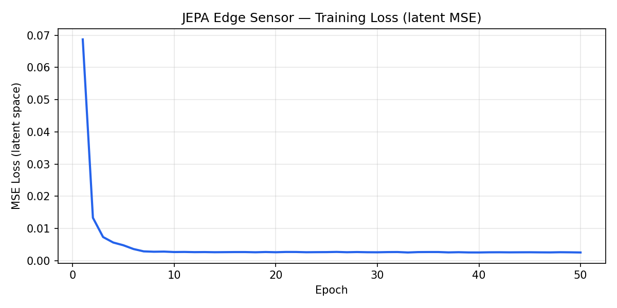 Latent MSE drops sharply from ~0.07 in the first epoch to ~0.003 by epoch 10, then holds a stable floor through epoch 50.
The model learns the structure of the embedding space in the first 10 epochs. The remaining 40 epochs are refinement. This is consistent with what you would expect from a small model on structured synthetic data: the capacity is sufficient, and the learning signal is clean.
Results
| Metric | Value |
|---|---|
| Final training loss (latent MSE) | 0.002582 |
| Mean inference latency | ~1.0 ms / step |
| Peak memory (Python heap) | 0.17 MB |
| Total parameters | 7,376 |
| Training epochs | 50 |
0.17MB peak memory. The Jetson Orin Nano has 8GB. This experiment uses roughly 0.002% of that. That headroom matters: in a real edge deployment, the remaining memory is available for sensor drivers, preprocessing pipelines, communication stacks, and whatever else the system needs to run.
1ms inference latency. Real-time capable at 1-second sensor sampling intervals with three orders of magnitude of headroom.
Predicted vs Actual
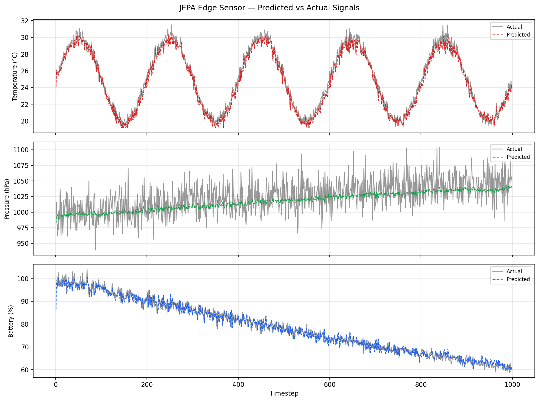
Three signals, three different behaviors:
Temperature tracks almost perfectly. The predicted curve hugs the sinusoidal actual signal tightly across all 1000 timesteps, including the peaks and troughs. The model has clearly learned the periodic structure of this signal in latent space.
Pressure shows the most interesting behavior. The actual signal has significant high-frequency noise on top of the underlying linear drift. The predicted curve tracks the drift but smooths out the noise entirely. This is not a failure. It is the right behavior for an edge monitoring system. The noise is not signal; the drift is. The latent representation has separated them.
Battery tracks the exponential decay closely, with the predicted and actual curves nearly indistinguishable across the full 1000-step range. The model correctly captures the monotonic decay structure from early in training.
What the Vector Store Adds
The cosine-similarity retrieval step is worth examining separately. At each inference step, the model retrieves the most similar past embedding from the 50-step rolling buffer and concatenates it with the current embedding before prediction.
For periodic signals like temperature, this retrieval tends to surface embeddings from approximately one period ago, states that are structurally similar to the current state. This gives the predictor implicit phase information without any explicit recurrence or positional encoding.
For monotonic signals like battery, the retrieved embedding is typically recent (the most similar past state is usually just a few steps back). The retrieval here acts more like a smoothing prior than a phase reference.
This is the LangGraph-style pattern applied to a minimal edge setting: a memory node that retrieves relevant context rather than maintaining a full hidden state. No recurrence, no attention, no additional parameters beyond the buffer itself.
Honest Caveats
Synthetic data is clean. Real edge sensors have non-stationary noise, calibration drift, missing readings, and interference from neighboring hardware. The model was not tested against any of these. The pressure smoothing result is encouraging but would need validation on real sensor data before drawing strong conclusions.
The linear encoder is a deliberate simplification. A linear encoder makes the embedding space interpretable and the pseudo-inverse decoding tractable, but it limits the expressiveness of the latent representation. A nonlinear encoder would likely improve prediction quality at the cost of losing the clean analytical inverse.
The vector store is in-memory. On a Jetson with limited memory, a 50-step buffer of 16-dimensional float32 embeddings costs about 3.2KB, which is negligible. Scaling the buffer size or embedding dimension would require more careful memory accounting.
Why This Matters for Edge AI
The dominant narrative in AI hardware is about scaling up: more memory, more compute, faster interconnects. That narrative is correct for foundation models. It is not the only story.
There is a large class of real-world deployments where the hardware is fixed and small, the task is local and continuous, and the value is in reliable real-time inference rather than occasional high-complexity reasoning. Industrial monitoring, autonomous robotics, environmental sensing, wearables. These systems run on Jetson-class hardware or smaller, and they run for months or years without interruption.
For those deployments, a 7,376-parameter model that runs in 1ms and uses 0.17MB is not a toy. It is a practical building block. The JEPA framing (learning structure in latent space rather than mapping raw inputs to raw outputs) makes it more robust to noise and more generalizable across operating conditions than a naive regression model of the same size.
That is what this experiment is pointing toward. Smaller systems that can quietly learn and adapt at the edge.
Resources
| Resource | Link |
|---|---|
| Code | hellojais/jepa-edge-sensor |
| Dataset | sensor_dataset.csv |
| JEPA (LeCun, 2022) | A Path Towards Autonomous Machine Intelligence |
Reach out at hellojais@gmail.com or @hellojais on GitHub if you have run similar experiments on Jetson-class hardware.