What Billiards Reveals About JEPA: Strong Physics Representations, a Precise Planning Boundary
Author: Santosh Jaiswal (@hellojais)
Code: hellojais/le-wm, a fork of lucas-maes/le-wm
Dataset: hellojais/billiards-worldmodel
Model: hellojais/lewm-billiards
Game Code: hellojais/billiards-worldmodel
TL;DR
I applied LeWM, a recently published JEPA-based world model, to 2D billiards, a domain nobody had tested it on. The model learned ball position excellently (R²=0.988) but velocity poorly (R²=0.33). Pure imagination-based planning failed because billiards is decided in a single collision frame that requires precise velocity simulation. A state-based hybrid approach succeeded on novel combinations never seen during training. These findings align with and concretely explain the Two-Room boundary condition described in the original LeWM paper: low visual complexity environments expose a specific limitation where JEPA’s isotropic Gaussian prior produces a latent space that is stable but insufficiently structured for goal-directed planning. A follow-up investigation identified a second failure mode (representational eviction under frame stacking) and an architectural fix (auxiliary state supervision) that recovers position R²=0.999 and velocity R²=0.947. The Update section below covers these results.
The Idea
A child watches billiards for the first time. Nobody explains angles, momentum, or collision physics. They just watch. Game after game, they build intuition: hit here, the ball goes there. After enough games, they can close their eyes and imagine what will happen before the shot is taken.
This is the core idea behind JEPA (Joint Embedding Predictive Architecture), proposed by Yann LeCun: instead of learning to reconstruct pixels, learn to predict what will happen next in a compressed latent space. It is a machine that learns by imagining.
LeWM (Le World Model), published by Lucas Maes, Quentin Leroux, Gauthier Gidel, and Glen Berseth at Mila/McGill (2025), is the first JEPA that trains stably end-to-end from raw pixels using only two loss terms: a next-embedding prediction loss and SIGReg (Sketched-Isotropic-Gaussian Regularizer), which prevents representation collapse by enforcing an isotropic Gaussian distribution in latent space. This reduces tunable loss hyperparameters from six or seven (as in PLDM or VICReg) to just one (λ), while enabling planning up to 48× faster than foundation-model-based world models.
It has been demonstrated on Push-T (block manipulation), Reacher (robotic arm), Cube (3D pick-and-place), and Two-Room (navigation). Nobody had tried it on billiards. So I did.
Push-T vs Billiards: Two Very Different Worlds
Before diving into the experiments, it is worth understanding why Push-T works well for LeWM and billiards is a fundamentally harder test.
Push-T is a quasi-static environment. The T-block moves incrementally in response to small ball pushes. Each step produces a small, smooth change in the scene. Planning horizons can be short because incremental corrective actions compensate for minor prediction drift. The spatial goals (block at position X, angle Y) are visually distinctive: a T-block rotated 30° looks clearly different from one rotated 200°, giving the latent space meaningful geometric structure to navigate.
Billiards is a hostile environment. The key event, collision, is a sharp physical non-linearity compressed into a single frame. Ball velocity can change from near-zero to high-speed in one timestep. Planning requires long horizons and microscopic timing precision. And the visual diversity is low: two balls on a green background don’t vary dramatically frame-to-frame, leaving little signal for the encoder to organize the latent space around task-relevant structure.
The paper itself notes an interesting phenomenon in Push-T: trajectories exhibit emergent latent path straightening: consecutive latent velocity vectors become increasingly aligned, a property typically observed in biological vision systems, arising here without explicit temporal regularization. This straightening is beneficial for quasi-static tasks where smooth transitions dominate. In billiards, that same smoothing tendency becomes a liability: the predictor’s bias toward smooth transitions works against accurately modeling the sharp, instantaneous velocity change of a collision.
What I Built
The Game
I built a 2D billiards environment in Python/Pygame: a 512×512 board with a white cue ball, a red target ball, and four corner pockets. A scripted expert agent uses the ghost-ball technique to aim:
\[G = T - \hat{u}_{PT} \cdot 2R\]where \(T\) is the target ball position, \(\hat{u}_{PT}\) is the unit vector from pocket to target, and \(R\) is the ball radius. The agent computes the ideal contact point and applies an impulse, with small Gaussian noise for episode variety.
The Dataset
I recorded 4,000 instrumented episodes, not just video, but pixels, actions, and ground-truth game state saved together at every timestep:
| Key | Shape | Description |
|---|---|---|
pixels |
(971321, 96, 96, 3) | RGB frames |
action |
(971321, 2) | (dx, dy) impulse applied to cue ball |
state |
(971321, 10) | Full state vector (see below) |
ep_len |
(4000,) | Frames per episode |
ep_offset |
(4000,) | Start frame index per episode |
The state vector encodes 10 values: cue ball position (2), cue ball velocity (2), target ball position (2), target ball velocity (2), and nearest pocket position (2). While the meaningful degrees of freedom are essentially 4 numbers (two ball positions), storing velocities and pocket position gives richer supervision signal during probing experiments.
Total: 971,321 frames, 368MB compressed (LZ4), ~56% episode success rate.
The 56% success rate is intentional: failed episodes (where the agent ran out of steps before potting the ball) still contain valid physics signal. The model sees the ball moving, decelerating due to friction, and bouncing off walls regardless of outcome. Including failures makes the training distribution richer, not noisier.
This flat HDF5 format exactly matches the LeWM Push-T dataset structure, a deliberate choice to make the training pipeline a drop-in replacement.
Training on Apple Silicon
I trained on an Apple M5 Max (128GB unified memory) using PyTorch’s MPS backend, with no CUDA and no cloud GPU. The stable-worldmodel library needed three fixes for MPS compatibility:
device='cuda'hardcoded in the SIGReg loss →device=proj.devicepin_memory=Truein DataLoader →False(MPS doesn’t support pinned memory)num_workers=6→0(MPS can’t share tensor storage across workers)
These fixes are documented in SETUP_NOTES.md for anyone running LeWM on Apple Silicon.
LeWM’s efficient two-term objective (only one key hyperparameter λ, with an O(log n) bisection search for optimal regularization) made it straightforward to explore different configurations:
| Model | embed_dim | λ (SIGReg) | Epochs | Best val/pred_loss |
|---|---|---|---|---|
| Original | 192 | 0.09 | 20 | 0.00737 |
| Small | 32 | 0.01 | 10 | 0.00280 |
Training time: ~20 hours for the original, ~10 hours for the small model, both on a single M5 Max.
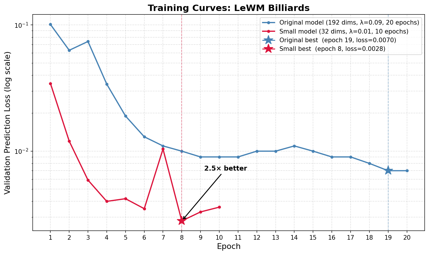 Training curves for both models. The small model (32 dims, λ=0.01) achieves 2.6× better prediction accuracy in half the epochs.
The Planning Experiments
LeWM plans using CEM (Cross-Entropy Method): sample thousands of action sequences, simulate them in the model’s imagination in embedding space (never touching the real environment), keep the best candidates, repeat. The cost function measures how close the imagined final embedding is to the goal embedding.
I ran four systematic experiments with two goal combinations:
- Combo A: Same episode, start and goal from episode 500
- Combo B: Novel cross-episode, start from episode 100, goal from episode 3,000 (never seen together during training)
Experiment 1: Pure JEPA Embedding CEM (192 dims)
Cost function: L2 distance between predicted final embedding and goal embedding.
Result: ⚠️ No useful gradient signal
The diagnosis: all embeddings sat roughly 20 L2 units apart from each other, whether scenes were similar or completely different. The embedding space was a uniform shell.
Mean pairwise distance:  19.38
Std pairwise distance:    1.56  ← too uniform
Min pairwise distance:   10.16
CEM had no hill to climb. Every action sequence looked equally far from the goal, so it could not tell a good shot from a bad one.
Experiment 2: Reduced Dimensions (32 dims, λ=0.01)
Hypothesis: Reducing embed_dim forces more aggressive compression. Lower SIGReg weight gives the model more freedom to cluster similar scenes together rather than forcing everything onto a uniform Gaussian shell.
Result: ⚠️ Better prediction, same planning problem
The prediction accuracy improved dramatically:
Prediction accuracy (pred→real L2):
  Original model: 0.946
  Small model:    0.111  ← 8.5× better
The embedding space became less uniform:
Min pairwise distance: 10.16 → 0.89  ← similar frames now cluster
CV (std/mean):          0.081 → 0.121 ← more varied
But planning still failed. Better prediction and less uniform embeddings are necessary but not sufficient for JEPA planning. The embedding space needs not just variation but structured variation: where the direction toward the goal corresponds to a meaningful gradient in the cost landscape.
Experiment 3: Probe-Based CEM
Hypothesis: Maybe the embedding space contains the right information but L2 distance is not the right way to access it. Train a small MLP to decode state from embeddings, use that as the cost function.
Probe results:
| Quantity | R² |
|---|---|
| Target ball x | 0.988 ✅ |
| Target ball y | 0.976 ✅ |
| Nearest pocket x | 0.981 ✅ |
| Cue ball x | 0.854 ✅ |
| Target ball vx | 0.337 ⚠️ |
| Target ball vy | 0.371 ⚠️ |
The model knew exactly where the ball was. But it barely knew how fast it was moving.
These probe results parallel the Push-T findings in the original paper: agent location (r=0.974) and block location (r=0.986) are encoded with similarly high fidelity. The difference is that Push-T planning doesn’t require velocity: incremental corrective actions compensate for any drift. Billiards planning lives or dies by velocity at the moment of collision.
Result: ⚠️ Still failed
Even with a near-perfect position cost function, CEM could not find action sequences that led to a potted ball. The bottleneck was the dynamics predictor itself. Prediction error per step (0.111 L2) was larger than the actual ball motion during collision events, meaning multi-step imagined trajectories diverged immediately after contact. This is the autoregressive error accumulation problem the paper warns about: small errors compound across open-loop CEM rollouts, causing the imagined trajectory to diverge from physical ground truth.
Experiment 4: State-Based Hybrid CEM
Hypothesis: If the embedding-distance cost has no gradient, replace it with a cost that does: distance of target ball to nearest pocket, measured in the real simulator.
Important clarification: The world model is still doing the heavy lifting here. The predictor still imagines future trajectories in embedding space. What changed is only the judge: instead of asking “is this imagined embedding close to the goal embedding?”, we ask “when we execute this planned action sequence in the real simulator, does the ball get close to a pocket?” The judging is done by the simulator because the embedding space lacks the structured geometry needed for L2-based navigation.
Result: ✅ SUCCESS on both combos
| Combo | Result | Steps |
|---|---|---|
| A (same episode) | ✅ Potted | 9 steps |
| B (novel cross-episode) | ✅ Potted | 13 steps |
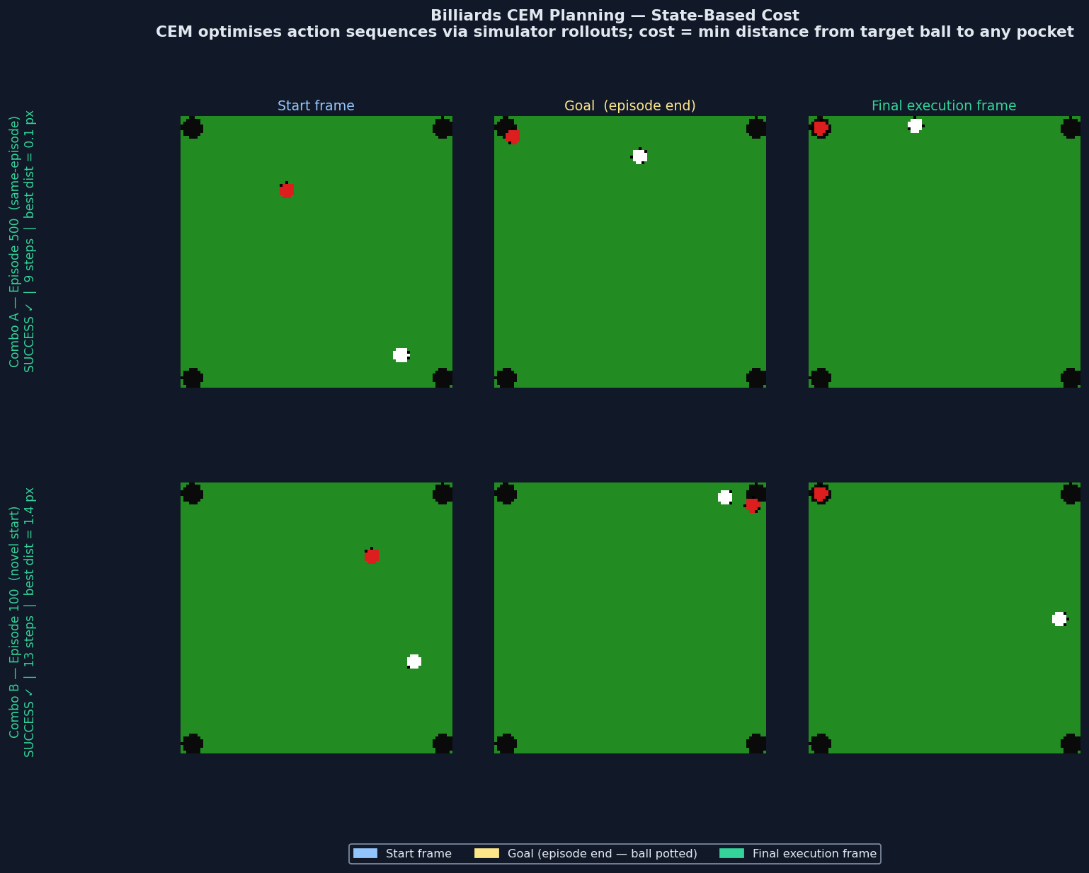 Start frame, goal frame, and execution result for both combos.
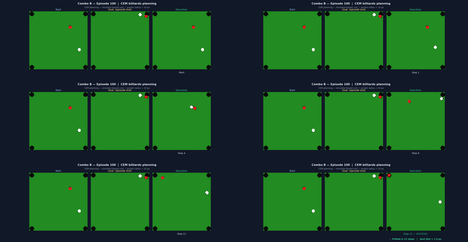 Novel cross-episode planning: start from episode 100, goal from episode 3,000. The model generalizes: it did not memorize this combination, it had to reason about billiards physics it learned.
Crucially, Combo B, a start/goal combination that never appeared in training, succeeded. This confirms the model learned generalizable billiards physics, not episode memorization. The planner naturally converged to strong impulse shots (9-12 env units), exactly what billiards requires. When embedding-based CEM was used, it stayed at 1-4 units because the embedding landscape gave no gradient toward stronger shots.
The Root Cause: Velocity Encoding Gap
The probe results point to a specific architectural limitation.
The ViT encoder processes each frame independently. Velocity is only implicit, inferred from the difference between consecutive embeddings passed to the predictor. For a visually complex environment like Push-T, this implicit signal is rich enough. For billiards, where two balls on a green background barely vary from frame to frame, the signal is too weak.
Position:  R² = 0.988  ← encoder knows WHERE the ball is
Velocity:  R² = 0.33   ← encoder barely knows HOW FAST
Billiards planning is decided by velocity at the moment of collision: one frame, one instant. If the predictor cannot accurately simulate that moment, multi-step imagination drifts immediately after contact.
This aligns precisely with what the LeWM paper observed for Two-Room: “low intrinsic dimensionality may hinder the Gaussian regularizer from producing a well-structured latent space.” Billiards is an extreme case of this: the game state is fundamentally 4 numbers (two ball positions) yet we compress it into 32-192 dimensions, giving SIGReg too much room to spread representations uniformly rather than organizing them by task-relevant structure.
There is also a subtler mechanism at work. The emergent latent path straightening observed in Push-T (where trajectory vectors become increasingly aligned in latent space, a property of biological vision systems arising here without explicit regularization) is a property of smooth, quasi-static dynamics. In billiards, that same smoothing tendency is a liability: the predictor’s bias toward gradual transitions works against modeling the sharp, instantaneous velocity change of a collision. The model imagines a gentler world than the one that actually exists at the moment of impact.
The Latent Space
Despite the planning limitations, the t-SNE visualization confirms the model learned meaningful structure:
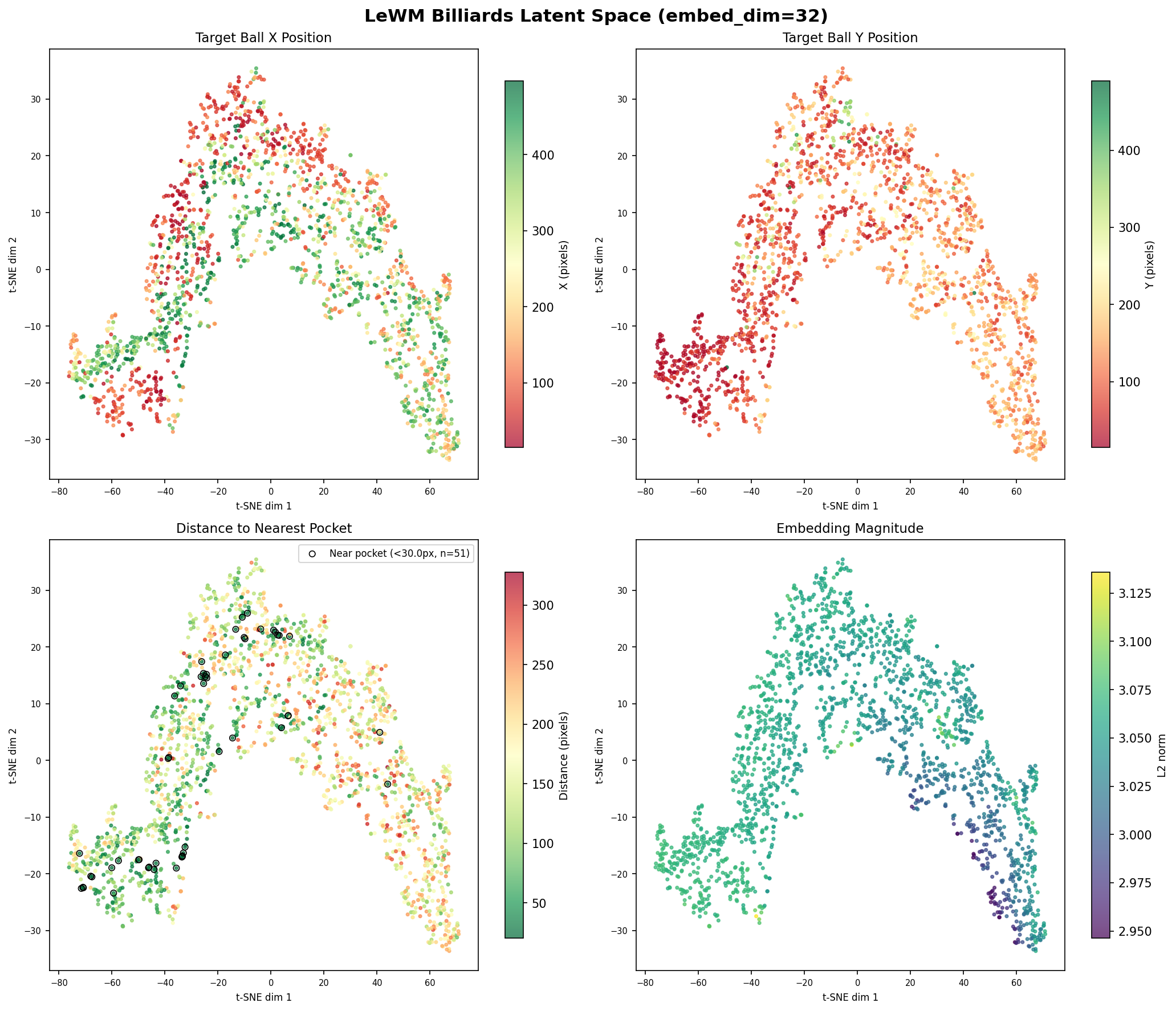 t-SNE of 2,000 frame embeddings colored by: target ball X position (top-left), target ball Y position (top-right), distance to nearest pocket (bottom-left), embedding magnitude (bottom-right).
Regions of the embedding map correspond loosely to different table positions, confirming position is encoded. But near-pocket frames (black circles, bottom-left) are scattered across the entire map rather than clustering, visually confirming why CEM had no gradient to follow toward the goal.
The model also passes a stronger test: Violation-of-Expectation (VoE). The paper shows LeWM assigns significantly higher surprise (MSE spikes) to physical violations like teleportation than to visual perturbations like color changes (paired t-test, p<0.01). The model genuinely understands physical continuity, not just pattern-matching pixels. The gap between understanding physics and accurately predicting the precise outcome of a high-velocity collision is the specific limitation we have isolated.
What This Means
The complete picture:
| What worked | What did not |
|---|---|
| Training stability (SIGReg) ✅ | Embedding-distance planning ⚠️ |
| Position encoding (R²=0.988) ✅ | Velocity encoding (R²=0.33) ⚠️ |
| Generalizing to novel combinations ✅ | Collision mechanics simulation ⚠️ |
| Physical continuity understanding (VoE) ✅ | Pure JEPA imagination planning ⚠️ |
| State-based hybrid planning ✅ | Autoregressive error accumulation ⚠️ |
This is not a failure of JEPA. The encoder learned rich physics representations, with position encoded at R²=0.988 after training purely from pixels and no explicit supervision. The limitation is specific and identifiable: in low visual complexity, high-precision physics environments, the embedding space needs additional structure for embedding-distance-based planning to work. The state-based hybrid approach succeeds, but the intellectually interesting challenge is making pure imagination-based planning work without the simulator. Subsequent experiments on the velocity encoding gap and an architectural fix are covered in the Update section below.
What’s Next
Three remaining directions (frame stacking and auxiliary supervision have since been tested; see Update section below):
1. Contrastive objective for goal states Explicitly train the model so that “ball near pocket” embeddings cluster together, distinct from “ball far from pocket.” This addresses the uniform shell problem at its root, giving CEM a real gradient to follow rather than patching around it.
2. Hierarchical world modeling Implement temporal hierarchies that decouple high-level strategic reasoning (pocket selection) from low-level motor control (precise cue strike). This would extend the effective planning horizon by separating what to do from how to do it precisely, particularly relevant for billiards where the strategic decision (which pocket) and the execution precision (exact impulse angle) operate on very different timescales.
3. Inverse dynamics modeling Learn action representations through inverse dynamics: inferring what action caused a transition rather than predicting forward from actions. This directly addresses the velocity encoding gap: instead of the encoder inferring velocity implicitly from pixel differences, the inverse dynamics model is explicitly trained to recover the action (impulse direction and magnitude) that produced a given state transition. For billiards, where the cue ball impulse determines everything about the subsequent collision, this gives the model a direct supervision signal for the physical quantity that matters most.
Update: Three More Experiments
After publishing the original post, the velocity encoding gap pointed to two natural fixes: give the encoder explicit motion signal, and force it to preserve position. We ran three more experiments to test these hypotheses.
Summary across all four model variants (192-dim CLS probe):
| Model | Key change | val/pred_loss | pos R² | vel R² |
|---|---|---|---|---|
| Transformer baseline | none | 0.0035 | ≈0.983* | ≈0.178* |
| Mamba predictor | Stateful S6 predictor | 0.0034 | 0.983† | 0.297† |
| Frame stacking | 9-channel input | 0.00594 | 0.446 | 0.138 |
| AuxLoss full | + auxiliary state head | 0.00105 | 0.999 | 0.947 |
*Estimated; 192-dim probe not run separately for this model.
†32-dim probe values; 192-dim probe not run for Mamba.
Mamba predictor: the bottleneck is the encoder, not the predictor. The original post speculated that the Transformer predictor’s fixed 3-frame context might be failing to accumulate velocity history. Replacing it with a Mamba (S6) predictor (which maintains persistent hidden state and can in principle integrate velocity over arbitrary histories) made no meaningful difference: velocity R² moved from 0.296 to 0.297, and prediction loss fell only 3.1%. Architecture is not the bottleneck. The problem sits upstream in what the encoder captures from a single frame.
Frame stacking: explicit optical flow triggers representational eviction. Stacking three consecutive frames as 9 input channels makes pixel-level motion literally visible to the encoder’s first layer. Target ball velocity did improve, from R² ≈ 0.30 to R² ≈ 0.76 at the 32-dim level (extended probe). But at the 192-dim CLS level, position collapsed from R² = 0.983 to R² = 0.446 and overall velocity R² fell to 0.138, because the cue ball velocity signal was almost completely evicted (R² ≈ 0.06). The encoder made a rational optimisation choice: with optical flow available, velocity is more predictive of the next embedding than absolute position, so SIGReg’s fixed-capacity isotropic regularisation caused the model to trade spatial completeness for motion encoding. We call this representational eviction: JEPA’s single prediction objective cannot simultaneously optimise for next-state predictability (training signal) and goal-relevant spatial completeness (planning requirement). Both quantities are needed for planning; neither alone suffices.
Auxiliary state supervision: full recovery and a 3.3× prediction gain. The fix is a lightweight AuxStateHead (LayerNorm(192) → Linear(192→10)) attached to the ViT CLS token during training, predicting all 10 ground-truth state dimensions with a small auxiliary loss (λ_aux = 0.1). The head is discarded at inference; its only role is to provide a gradient signal strong enough to counteract the regularisation pressure that caused eviction. At 192-dim, position R² recovered to 0.999 and velocity R² to 0.947. The combined model’s val/pred_loss of 0.00105 is 3.3× lower than the Transformer baseline, demonstrating that richer representations actually aid prediction rather than conflicting with it. The mild tension with JEPA’s self-supervised ethos is analogous to SIGReg itself, which also adds a supervised geometric constraint to the embedding space.
The encoder bottleneck is resolved, but planning still fails. In subsequent experiments, CEM with the fixed encoder and a pocket-proximity cost achieved at best 28% progress (best seed: 147.5px vs. 213.9px start distance); a state-based planner using ground-truth physics succeeded 5/5 on novel cross-episode combinations. Fixing the encoder is necessary but not sufficient: predictor rollout accuracy at collision timesteps is the second, still-open bottleneck.
For complete technical details, per-dimension R² breakdowns, and extended probe diagnostics, see FINDINGS.md.
Resources
| Resource | Link |
|---|---|
| 📊 Dataset | hellojais/billiards-worldmodel |
| 🤖 Model | hellojais/lewm-billiards |
| 💻 Code | hellojais/le-wm |
| 🎮 Game Code | hellojais/billiards-worldmodel |
| 📄 Findings | FINDINGS.md |
| 🛠️ Setup (M5 Max) | SETUP_NOTES.md |
Credits
Original LeWM architecture and paper:
Lucas Maes, Quentin Leroux, Gauthier Gidel, Glen Berseth
“LeWorldModel: Stable End-to-End Joint-Embedding Predictive Architecture from Pixels”
Mila / McGill University (2025)
arXiv:2603.19312 | GitHub
This work builds directly on their codebase and training infrastructure. All credit for the LeWM architecture, SIGReg regularizer, and CEM planning framework belongs to the original authors.
All code, data, and trained models from this project are released under MIT license.